
Learning to survive
On a previous post I made the case that survival analysis is essential for better churn prediction. My main argument was that churn is not a question of “who” but rather of “when”.
In the “when” question we ask when will a subscriber churn? Put differently how long does a subscriber stay subscribed on average? We can then answer one of the most important questions: What is the average subscriber life time value?
The survival curve
Let’s roll up our sleeves and dive right in: The survival curve \(S(t)\) measures the probability a subscriber will “survive” (not churn) until time \(t\) since starting his subscription. For example \(S(3)=0.8\) means a subscriber has %80 chance of not churning by the \(3^{rd}\) month of subscription.
The most common way of estimating \(S(t)\) is by using the Kaplan-Meier curve who’s formula is given by:
\[\hat{S}(t) = \Pi_{t_i \leq t}\left(1-\frac{d_i}{n_i}\right)\] where \(t_i\) are all times where at least one subscriber has churned, \(d_i\) is the number of subscribers who have churned at time \(t_i\) and \(n_i\) is the number of subscribers who survived till at least \(t_i\). The term \(\frac{d_i}{n_i}\) is then the probability of churning at time \(t_i\).
To illustrate let’s calculate the survival curve for the following subscriber data:
| subscriber | t | churned |
|---|---|---|
| 1 | 3 | 0 |
| 2 | 6 | 1 |
| 3 | 2 | 1 |
| 4 | 1 | 0 |
| 5 | 2 | 0 |
| 6 | 2 | 1 |
The column \(t\) denotes the time a user has been subscribed until today. If he churned that would be the time till he churned.
We have 2 times at which churn events happend: \(t_i = \{2,6\}\).
For \(t < 2\) we have \(S(t)=1\) since no one churned up to that point.
At \(t_1=2\) we have \(d_1=2\) (subscribers 3 and 6) and \(n_1=5\) (all subscribers but 4). Using the above formula we get:
\[S(2) = 1-\frac{2}{5} = 0.6\]
At \(t_2=6\) we have \(d_2=1\) (subscriber 2) and \(n_2=1\) (again, just subscriber 2).
We thus have:
\[S(6) = \left(1-\frac{2}{5}\right) \cdot \left(1-\frac{1}{1}\right) = 0\]
Let’s plot that curve:
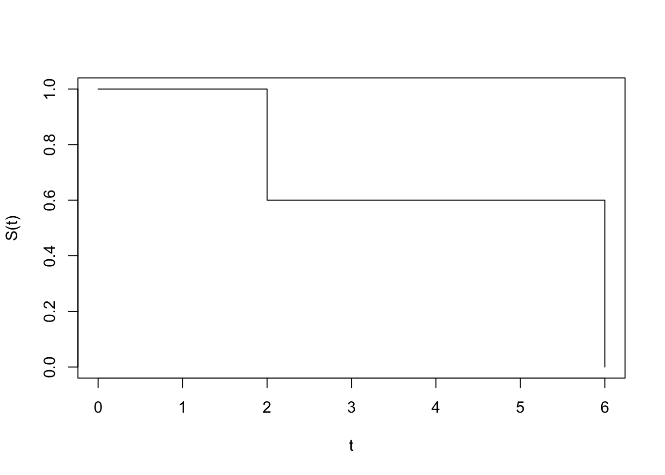
One thing to notice here is that at that every point along the curve we only consider subscribers who survived up to that point. If a subscriber joined very recently (e.g. subscriber 4) he won’t play a major role in the calculation.
In practice you’d be better off using the survival curve implementation in the R survival package or the python lifelines library.
Expected life time
So why go through the hassle of calculating \(S(t)\) in the first place? Turns out that the expected life time is the area under the survival curve (I won’t go into proving that here). If we denote the time at which a subscriber has churned by \(T\) then:
\[E(T) = \int_0^{\infty}S(t)dt\] And in our example above: \(E(T) = 2\cdot 1 + 4 \cdot 0.6 = 4.4\). If a users’ monthly plan bill is for example $10 then we can say that his expected LTV (life time value) is $44.
Better answering the “who” question
Sometimes we may actually be interested in the “who” question. On my next post I’ll show that using survival curves we can better answer that question as well!