Better churn prediction

To churn or not churn? - That is not the real question!

One of the main topics I’ve been working on through the years is churn. Churn reduction is a top priority for many companies and correctly identifying it’s root causes can greatly improve their bottom line.

Considering how well known and appreciated the churn problem is I’m often perplexed by how badly it is modeled in practice.

Churn is often formulated as a question of “who’s most likely to churn?”. This question naturally lends itself to classification modeling.

I argue however that churn is not really a question of “who” will churn but rather of “when”.

This is an important distinction for 2 reasons:

1. Asking “who” will churn leads to biased modeling as will be demonstrated below.
   
2. In many cases a users’ value is highly dependent on how long he’ll stay subscribed. This can only be answered by asking “when” rather than “who”.

Cellphone subscribers example

Take for example the classic case of cellphone subscribers. They pay a monthly fee until some point in time in which they decide to terminate their contract (aka churn).

Eventually they’ll all churn: 30 years from now they will be either dead or use Holograms to communicate rather than a Cellphone.

Let’s visualize how typical subscriptions look like:

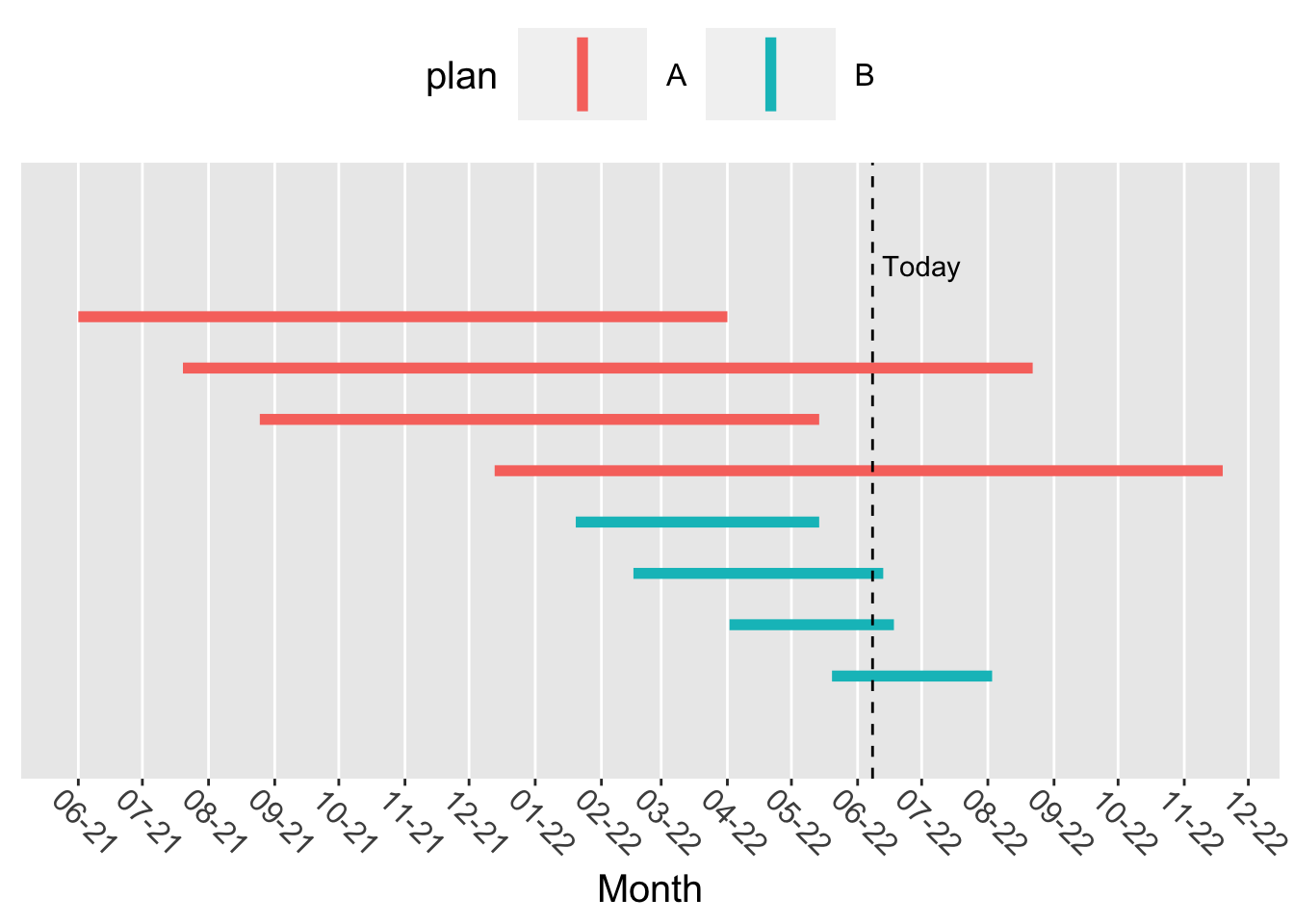
The first subscriber on the top started on plan A on June 2021 and churned on April 2022. The slashed line represents “Today” (the time the analysis is run) which is June 8th 2022.

In the “who” question, users who have churned in the past (before “today”) are labeled as “churned” (\(y=1\)) while those who churn in the future are labeled as “not churned” (\(y=0\)) since they are still subscribed when we observe them “today”.

We can see that users of plan A tend to take longer to churn (their lines are longer). But since they joined earlier than plan B subscribers they have more time to churn and will be labeled as “churned” more often (50% of plan A vs 25% in plan B).

We would thus wrongly conclude that plan A subscribers churn at a higher rate than plan B subscribers.

The bias illustrated above is very typical as cellphone plans are often introduced in succession. In the example above it can be seen that on January 2022 plan A was switched to plan B.

A small simulation study

To drive the point home I’ll conduct a tiny simulation analysis.

We have a timeline that starts at 0. The time we observe the data and fit our model (“today”) is 22.

The time a user started his subscription is drawn from a uniform distribution \(U~[0,20]\) if he’s on plan A and \(U~[20,22]\) if he’s on plan B.

today <- 22
Na <- 700
Nb <- 300
plan <- rep(c("A", "B"), time = c(Na, Nb))
set.seed(1)
join_time <- c(runif(Na, 0, 20), runif(Nb, 20, today))

Below we can see the average join time:

tapply(join_time, plan, mean)

##        A        B 
## 10.08968 20.97702

The time a user was subscribed before churning is distributed as Poisson with \(\lambda=4\) if he’s on plan A and \(\lambda=3\) if he’s on plan B.

set.seed(1)
time_to_churn <- c(rpois(Na, 4), rpois(Nb, 3))

Below we can see the average time to churn:

tapply(time_to_churn, plan, mean)

##        A        B 
## 4.045714 2.993333

The time a user churns is the time he joined + the time till he churned:

churn_time <- join_time + time_to_churn

If the churn time is greater than 22 (in the future from “today”) we say he’s not churned (\(y=0\)). If that time is shorter than today we day he did churn (\(y=1\)).

churned <- churn_time < today

Looking at raw churn rates we can see that users from plan A seem to churn much more:

tapply(churned, plan, mean)

##         A         B 
## 0.8042857 0.2233333

But we know users on plan B joined more recently so we’d might try to take that into account by fitting a logistic regression of churn vs plan and the time since a user joined.

Below we can see however that the bias is so strong that the model still tells us that being on plan B reduces the probability to churn:

time_since_join <- today - join_time
glm(churned ~ plan + time_since_join)

## 
## Call:  glm(formula = churned ~ plan + time_since_join)
## 
## Coefficients:
##     (Intercept)            planB  time_since_join  
##         0.19101         -0.02035          0.05149  
## 
## Degrees of Freedom: 999 Total (i.e. Null);  997 Residual
## Null Deviance:       233.1 
## Residual Deviance: 102.9     AIC: 572.3

What are we gonna do?

Use survival analysis!

To keep this post from getting too long I’ll skip introducing what survival analysis is and instead show how it handles the bias demonstrated above.

One common model in the survival analysis arsenal is the “Accelerated failure time” model. It produces coefficients much like a logistic regression:

library(survival)
observed_time <- ifelse(churned, time_to_churn, today - join_time)
# add a tiny amount (0.01) to observed_time to avoid observed_time = 0
survregExp <- survreg(Surv(observed_time + 0.01, churned) ~ plan,
  dist = "exponential"
)
coef(survregExp)

## (Intercept)       planB 
##   1.4558659  -0.2154432

We interpret the coefficients as follows: Being on plan B reduces time to churn by 20% (\(1 - exp(-0.2154432) = 0.2\)) compared with the population average. The average population time to churn is:

mean(time_to_churn)

## [1] 3.73

And the average time to churn in plan B is 3 which is indeed 20% lower than 3.7!

Conclusion

Asking the “when” question instead of “who” not only gives us unbiased results but also deeper insight into what we’re really interested with: How long do subscribers take to churn.

In the next few blog posts I’ll discuss survival analysis a bit more in depth and showcase advanced use cases in churn prediction where survival analysis is crucial for better churn modeling.