
Intro
We’ve seen on a previous post that one of the main differences between classic ML and Causal Inference is the additional step of using the correct adjustment set for the predictor features.
In order to find the correct adjustment set we need a DAG that represents the relationships between all features relevant to our problem.
One way of obtaining the DAG would be consulting domain experts. That however makes the process less accessible to wide audiences and more manual in nature. Learning the DAG from data automatically can thus make Causal Inference more streamlined usable.
On my last blog post we’ve hit a dead-end when it seemed non of the algorithms surveyed was able to learn the DAG accurately enough.
Enter: orientDAG package
While the algorithms surveyed on my last post were able to converge on the correct DAG skeleton (find edge presence without it’s orientation) they all failed in orienting the edges correctly. This means that for a given pair of variables X,Y the algorithms were able to tell if they are causally linked, but unable to determine if X causes Y or vice versa.
We can utilize literature centered around finding causal direction to correctly orient DAG edges after learning it’s skeleton.
When both X and Y are continuous, we can use the generalized correlation measure developed by Vinod.
When both X and Y are discrete, we can use the distance correlation measure (see Liu and Chan, 2016).
When either X or Y are discrete, and the other is continuous we can discretisize the continuous variable (using for example the procedure at infotheo::discretize) and use the method for 2 discrete variables mentioned above.
The orientDAG package uses the approach outlined above to orient DAG skeleton edges. To demonstrate how it works let’s go back to the example shown on my last post.
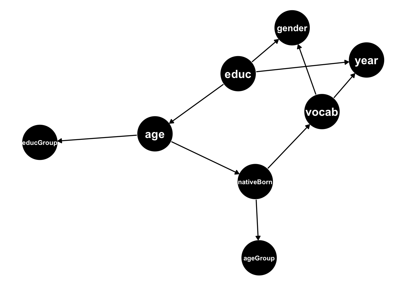
We used the simMixedDAG package to simulate datasets from the DAG below:
Following the bench-marking results on my last post we’ll restrict our attention to the bnlearn::tabu function for learning the DAG skeleton.
The main function in the orientDAG is fittingly called orient_dag. It takes as input an adjacency matrix where a 1 in the i,j position denotes an arrow from node i to node j.
Below we can see the adjacency matrix corresponding to the DAG above:
##            age ageGroup educ educGroup gender nativeBorn vocab year
## age          0        0    0         1      0          1     0    0
## ageGroup     0        0    0         0      0          0     0    0
## educ         1        0    0         0      1          0     0    1
## educGroup    0        0    0         0      0          0     0    0
## gender       0        0    0         0      0          0     0    0
## nativeBorn   0        1    0         0      0          0     1    0
## vocab        0        0    0         0      1          0     0    1
## year         0        0    0         0      0          0     0    0
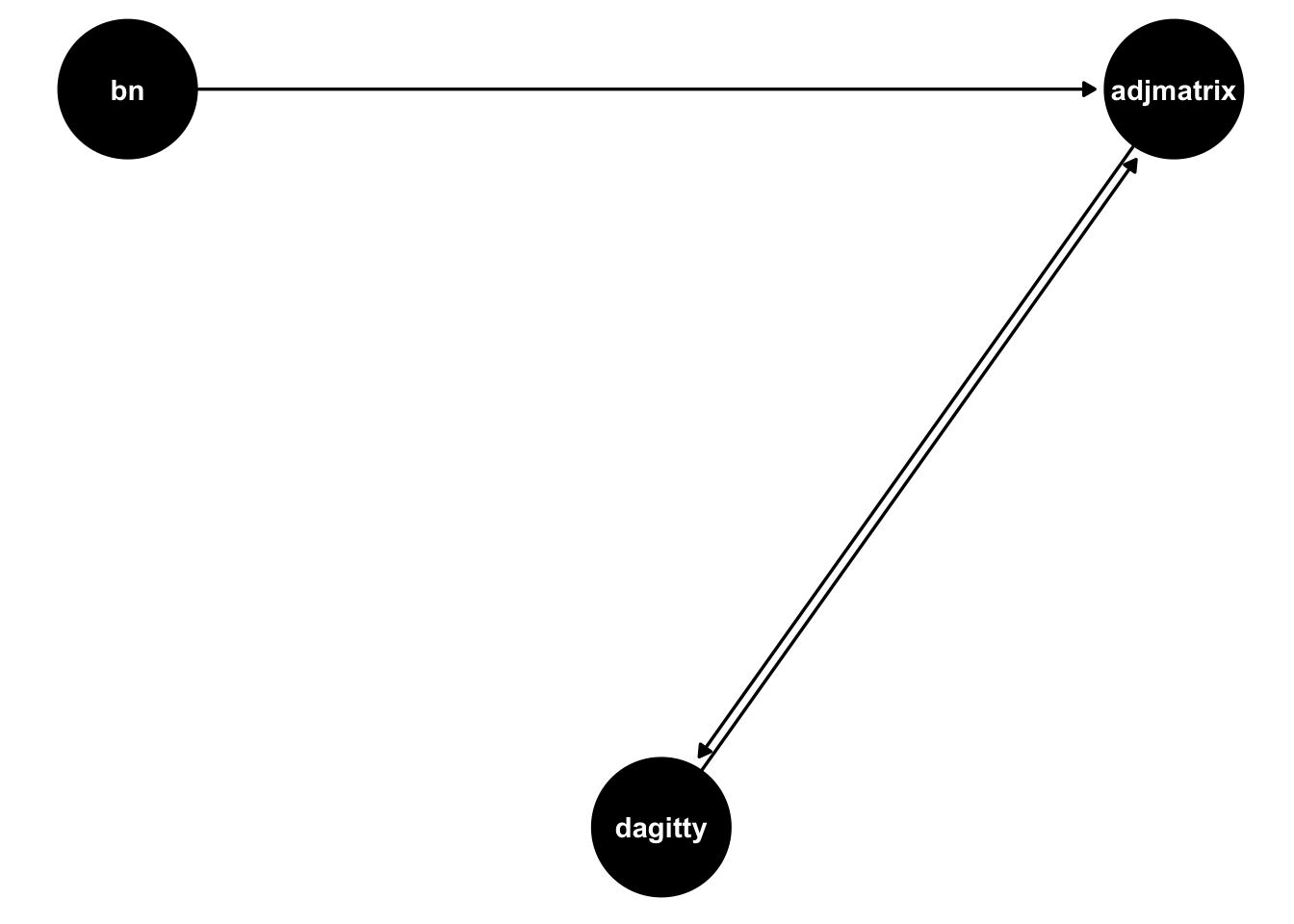
The package also contains utility functions that facilitate DAG conversion between different representations. We can thus take the fitted bn DAG object from the tabu function and convert it to an adjacency matrix using the function bn_to_adjmatrix. The DAG below shows all conversions available in the package:
As before, we’ll measure DAG learning accuracy by the Structural Intervention Distance. For every sample size \(n\) I simulate 100 datasets and measure SID. Below I compare the SID distribution for 3 algorithms:
- tabu: DAGs obtained using the tabu function from the bnlearn package
- tabu + orientDAG: DAGs obtained by further orienting the DAG’s from tabu using the orientDAG package
- random: DAGs obtained by randomly re-orienting the DAGs obtained by the tabu function
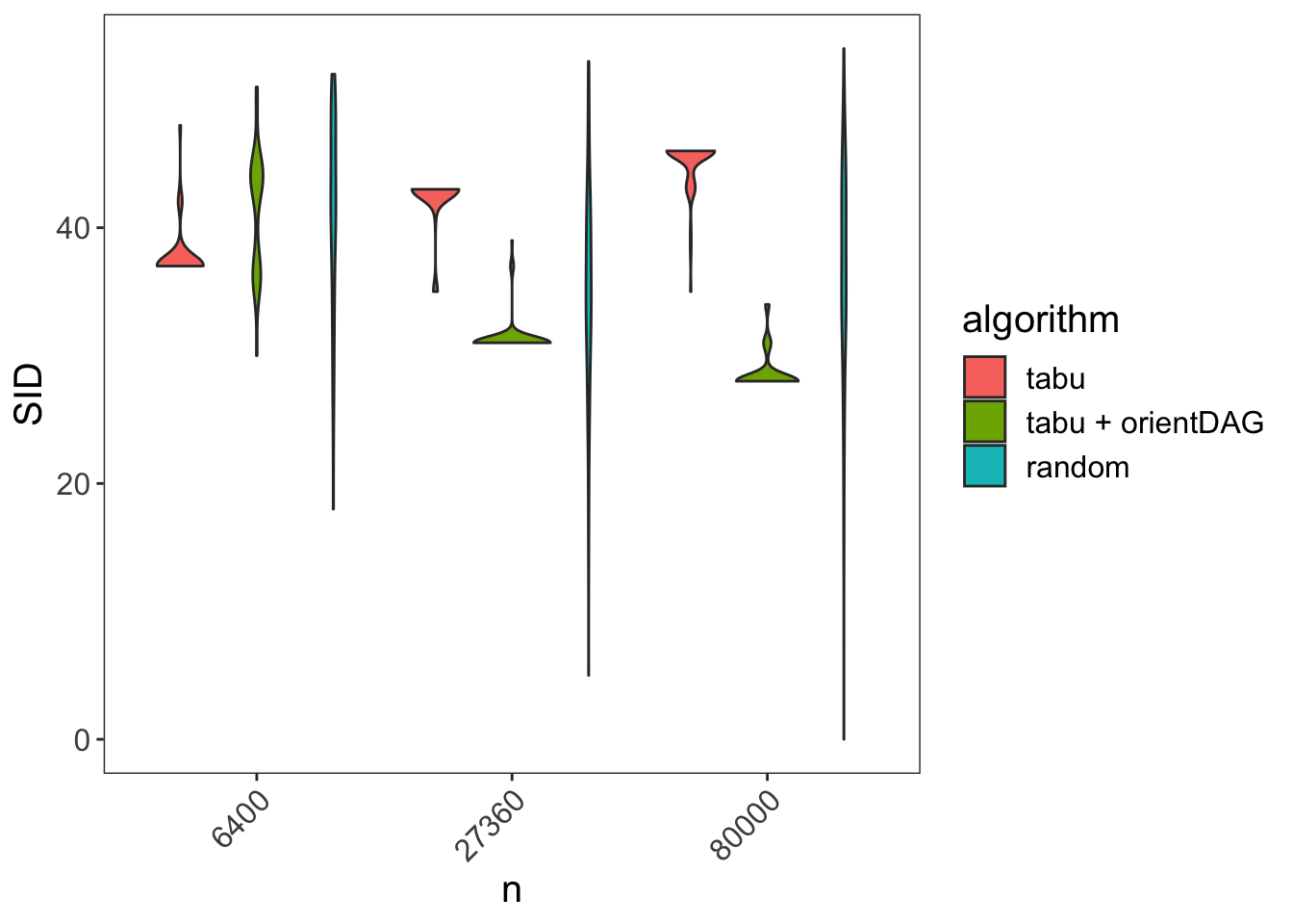
We can see that the tabu performance deteriorates as sample size grows while tabu + orientDAG improves.
From SID we can derive a more intuitive measure: The probability of finding the correct adjustment set for a randomly chosen pair of treatment-exposure variables:
\[P(\text{correct adj set)} = 1 - \frac{SID}{\#\{\text{possible treatment - exposure pairs}\}}\]
Below we can see the corresponding plot:
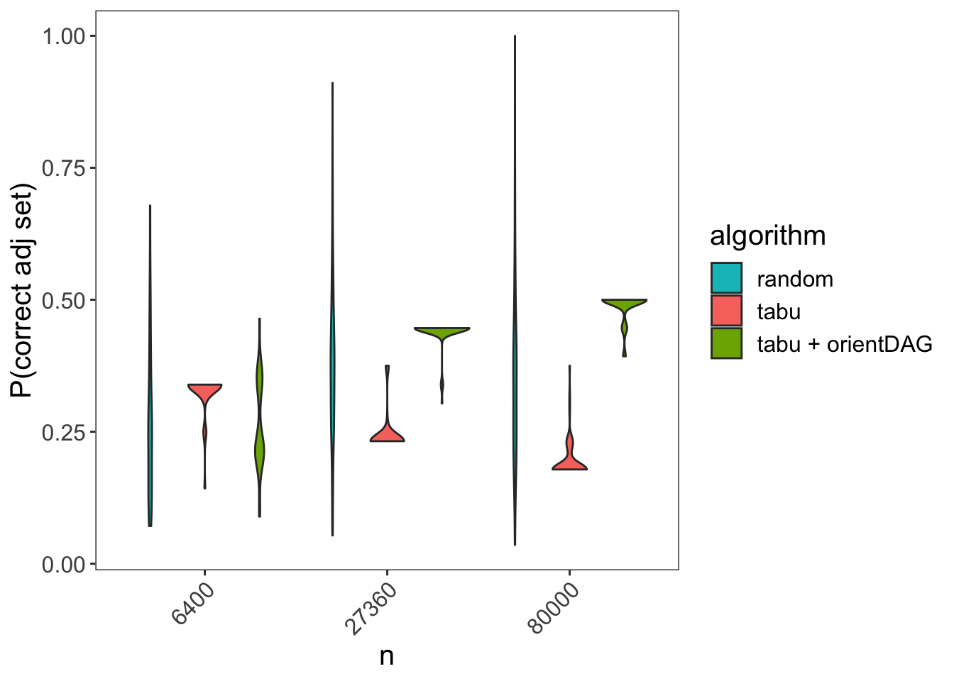
For \(n = 80,000\) the orientDAG package about doubles the performance compared with tabu.
Bayesian Network DGP
In the above example the underlying data generating process (DGP) didn’t conform to the Bayesian Network (BN) assumptions, which might explain the deteriorating performance of the tabu function.
Let’s see how the different algorithms fare when the underlying DGP does conform to the BN assumptions.
Below I plot the “mehra” DAG taken from the bnlearn package:
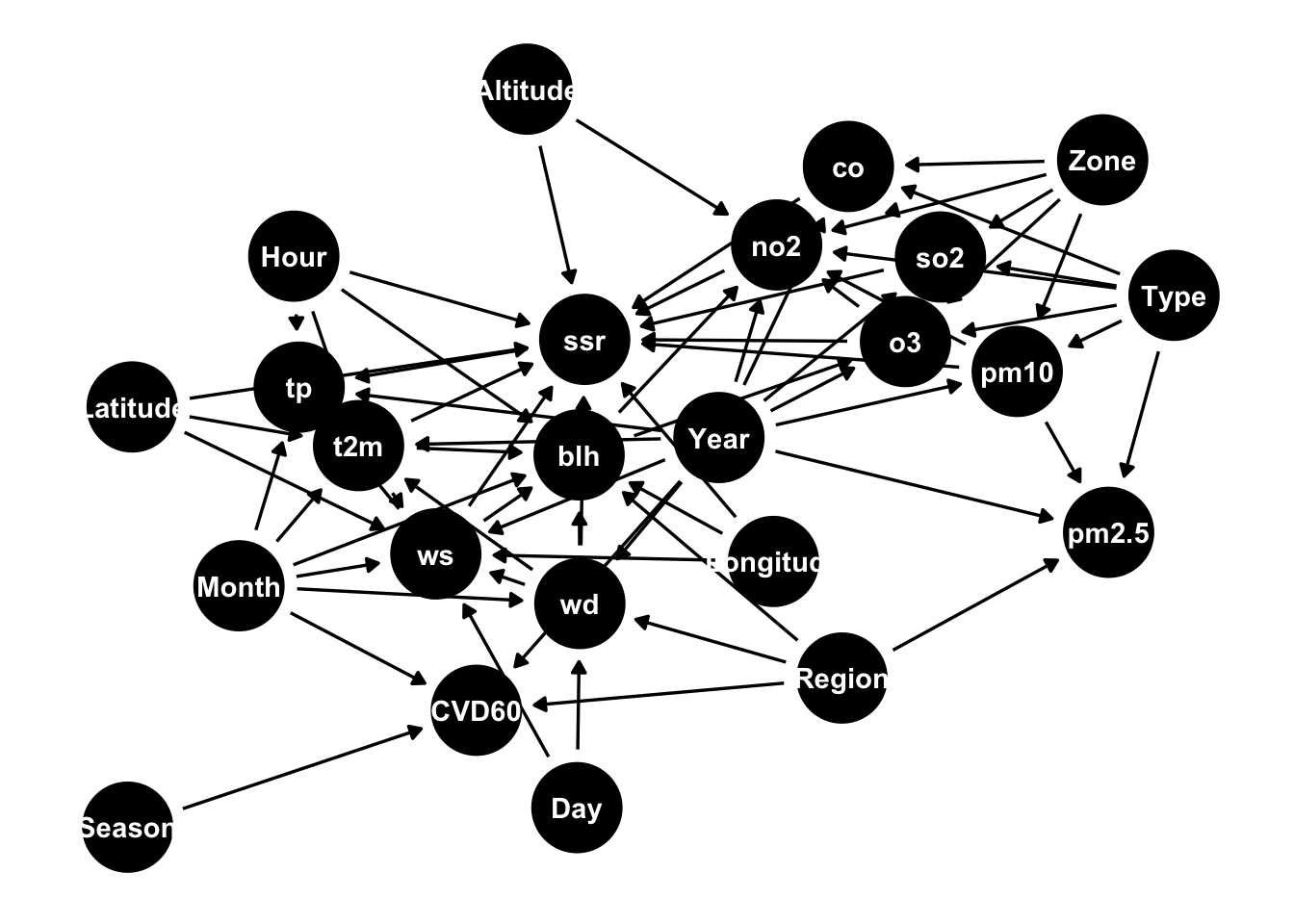
The above DAG contains 24 nodes, of which 8 are categorical. The nodes are connected by 71 arrows.
Below we can see SID for the different algorithms (this time running only 10 simulations per sample size due to the network size):
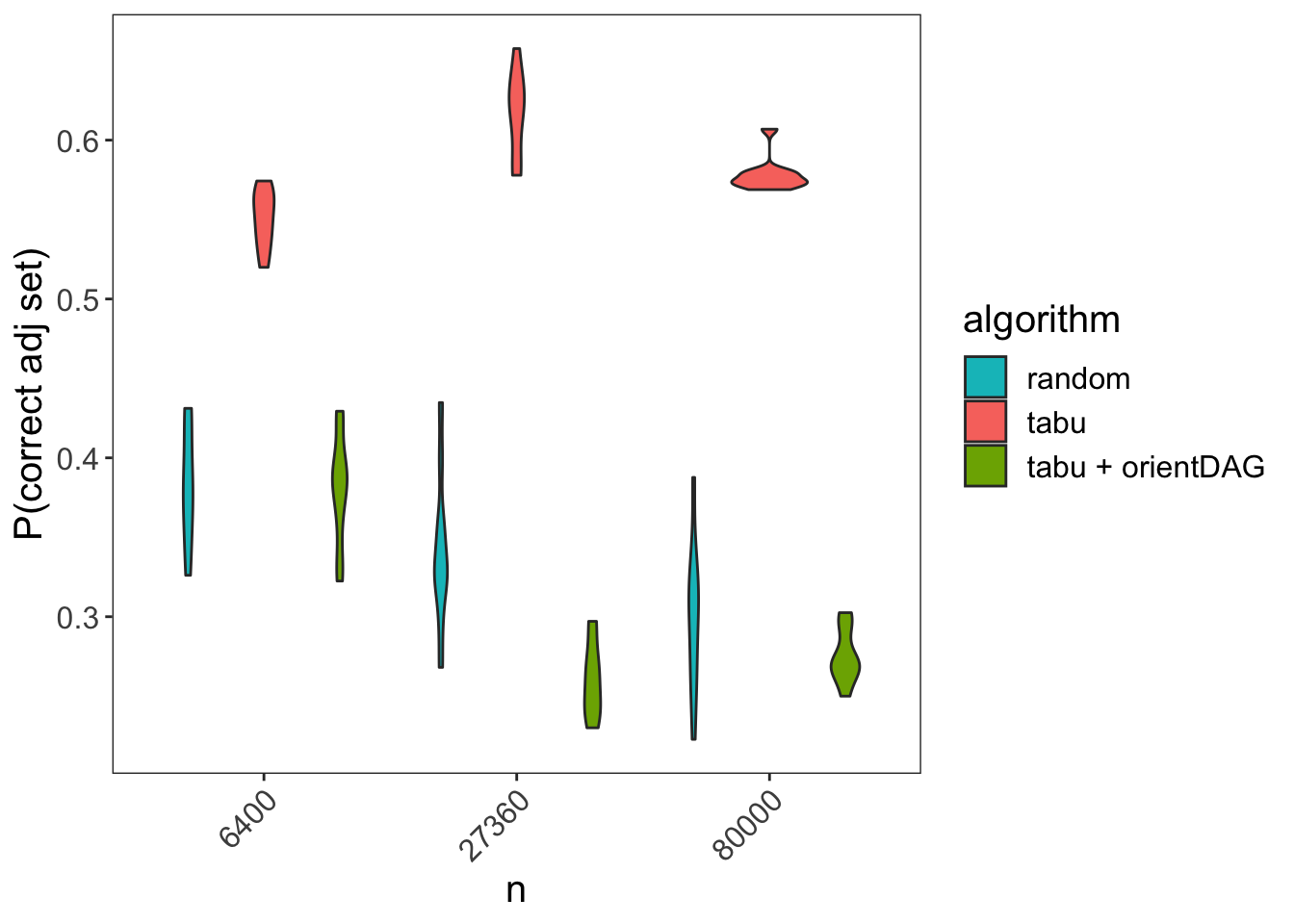
We can now see that when the BN assumptions hold the tabu function fares best as expected, while the tabu + orientDAG fares as bad as a random guess or even worse. It’s possible that the tabu + orientDAG performance is worse because it uses tests unrelated to the BN assumptions thus introducing noise to edges which are already oriented correctly by tabu.
We can mitigate such performance deterioration by introducing regularization parameters which force orient_dag to re-orient an edge only in cases where there is strong evidence for a given orientation. Namely, the difference between distance correlation/generalized correlations must exceed some threshold. We’ll call this approach tabu + orientDAG - conservative.
Below we can see the resulting performance measures:
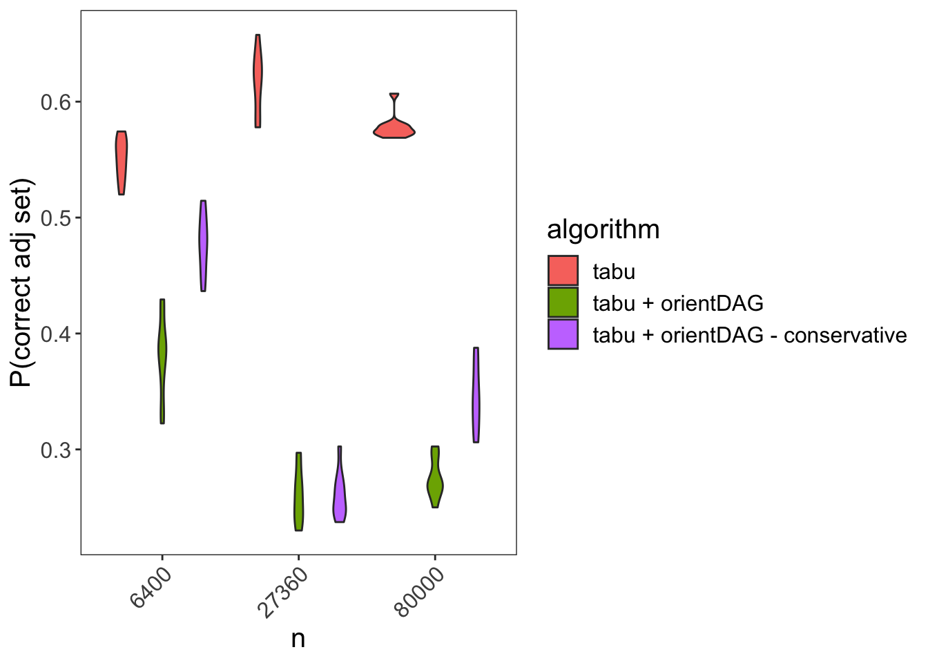
While the tabu + orientDAG still fares worse then tabu, it still is able to marginally at least outperform a random guess.
Conclusion
It would seem that automatic learning of DAGs is highly dependent on knowing the underlying DGP assumptions and also requires very large sample sizes - thus making automatic learning of DAGs unreliable (at least for the examples surveyed in this post).
It may be that a hybrid solution where some edges are white-listed (their presence and orientation are assumed known) and some are blacklisted (are assumed to be known not to exist) by an expert, followed by an automatic algorithm can produce more reliable results.