I was really struggling with finding a header pic for this post when I came across the one above - titled “Dag scoring and selection” and since it’s sort of the topic of this post I decided to use it!
Intro
On my second post I’ve stressed how important it is to use the correct adjustment set when trying to estimate a causal relationship between some treatment and exposure variables. The key to using the correct adjustment set is correctly identifying the underling DAG generating a dataset.
A few approaches I can think of to obtain a DAG for causal inference would be:
- Use domain knowledge and theory
- Pick one of a few candidate DAGs by comparing their fit to the data
- Use algorithms to automatically “learn” the underlying DAG
In this post I’ll explore the last approach. Being able to learn the underlying model DAG from a dataset “automatically” would enable non subject matter experts to do Causal Inference in a very similar fashion to classic ML.
Existing methods for learning DAGs
R has tons of packages for DAG estimation. Fortunately, the causalDisco is a great shiny app that enables searching DAG estimation functions using different criteria.
In this post I’ll restrict the discussion to the scenario where there are no hidden confounders and where the dataset contains both discrete (i.e. categorical) and numeric variables. We’d also like our estimation function to output a DAG with all edges oriented. Below we can see the results of applying these conditions in the causalDisco app:
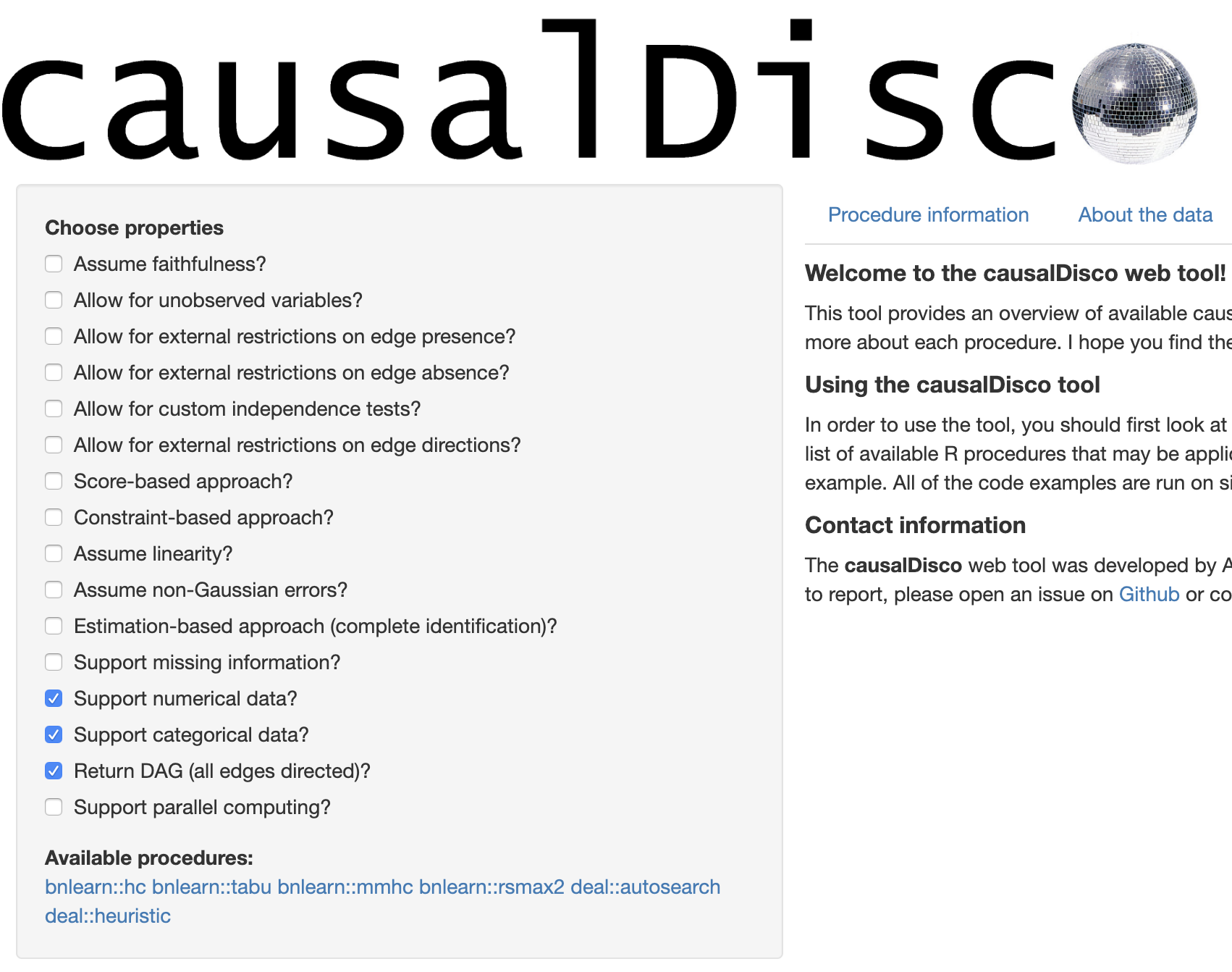
We get the following list: bnlearn::hc, bnlearn::tabu, bnlearn::mmhc, bnlearn::rsmax2, deal::autosearch and deal::heuristic.
After playing around a bit with the deal functions I found they were too manual for a quick algorithm comparison. I’ve thus decided to use only the bnlearn functions.
Estimated DAG dissimilarity measurements
How can we measure how different our estimated DAG is from the true DAG?
Edge distance
A simple way to measure estimated DAG dissimilarity with the true DAG would be to count how many edges are present in the true DAG yet missing in the estimated DAG and conversely, how many edges are present in the estimated DAG yet do not exist in the true DAG.
Let’s take as an example the DAG presented on my last post (presented on the left), along with an estimated DAG (on the right):
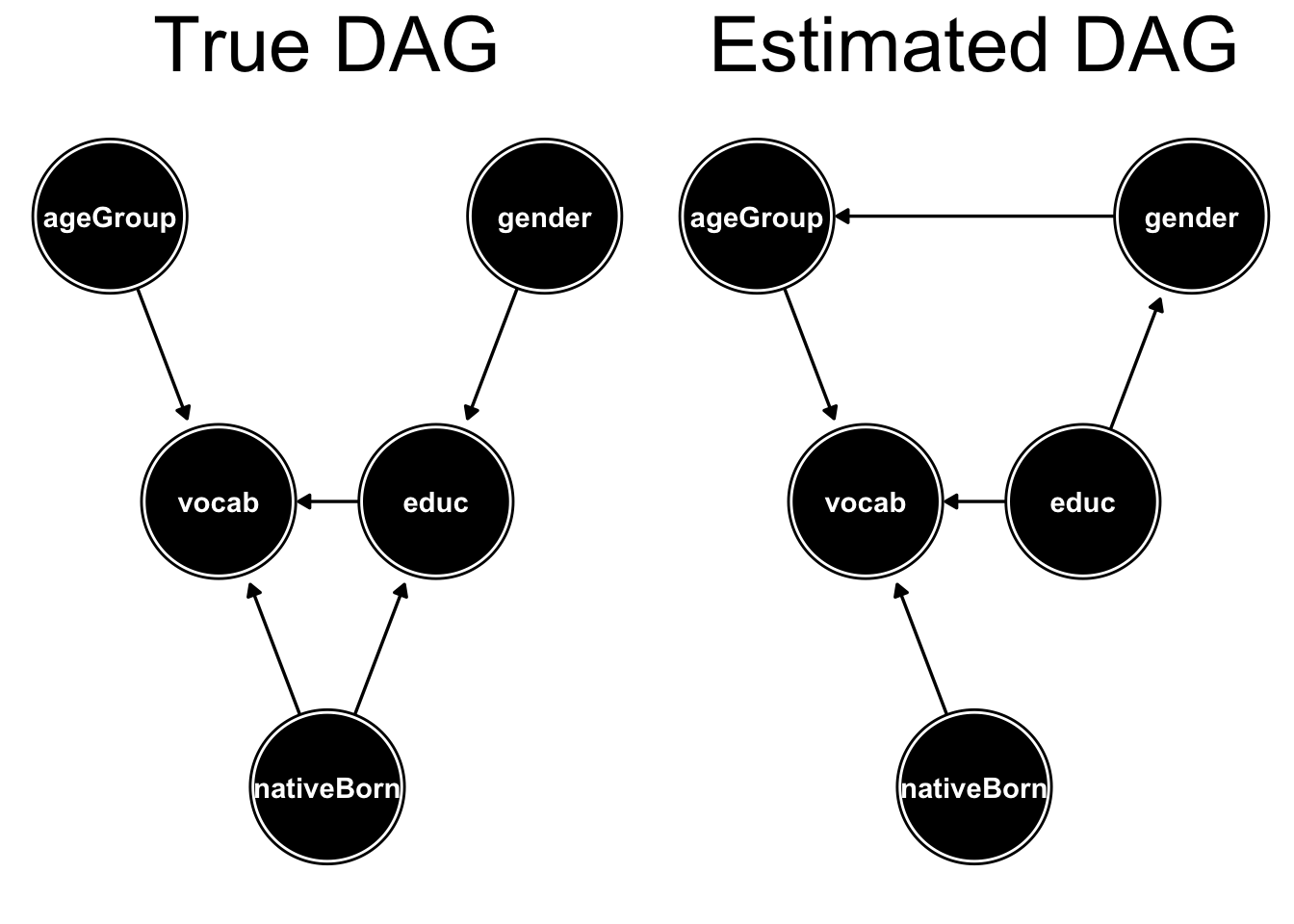
We can see in the above example that in the estimated DAG there’s an edge \(gender \rightarrow ageGroup\) which doesn’t exist in the true DAG, and that it’s missing the edge \(nativeBorn \rightarrow educ\). So the edge distance this case is 2.
Hamming distance
Even if an edge exists in the 2 DAGs, it would make sense to penalize it if the edge orientation is wrong. The Hamming distance is the same as the edge distance, only it counts in addition edges oriented incorrectly. In the above example we can see that the edge \(educ \rightarrow gender\) is oriented incorrectly (the true orientation is \(educ \leftarrow gender\)) and thus the Hamming distance in this case would be 3.
Structural Intervention Distance
The reason we construct DAGs to begin with is to enable correct adjustment set identification. It would thus make sense to measure DAG dissimilarity in light of that motivation.
To that end, the Structural Intervention Distance (SID) counts all possible treatment - exposure pairs where the estimated DAG does not yield a correct adjustment set.
To see the cases in the example above where the estimated adjustment sets are different than the true adjustment sets we can check the table below (we note an empty set {} means no conditioning is required to estimate the causal effect while “No adjustment sets” means there isn’t any set of variables we can adjust for to estimate the causal effect):
| treatment | exposure | True set | Estimated set |
|---|---|---|---|
| gender | educ | {} | No adjustment sets |
| educ | gender | No adjustment sets | {} |
| educ | nativeBorn | No adjustment sets | {} |
| gender | nativeBorn | {} | {} |
| educ | vocab | {nativeBorn} | {} |
| gender | vocab | {} | {educ} |
The SID in the example above would thus be 6.
DAG estimation algorithms benchmarking
In this section we’ll use the simMixedDAG package to simulate datasets from a DAG and benchmark different algorithms on recovering it using the above measures.
The DAG and data generating process (DGP) in this section will be based on the General Social Survey data.
The data structure is shown below:
| variable | class | sample_values | missing |
|---|---|---|---|
| year | numeric | Min. = 1978, 1st Qu. = 1988, Median = 1996, Mean = 1997.49, 3rd Qu. = 2008, Max. = 2016 | 0% |
| gender | factor with 2 levels | female, male | 0% |
| nativeBorn | factor with 2 levels | no, yes | 0% |
| ageGroup | factor with 5 levels | 30-39, 18-29, 60+, 40-49, 50-59 | 0% |
| educGroup | factor with 5 levels | 16 yrs, <12 yrs, 13-15 yrs, 12 yrs, >16 yrs | 0% |
| vocab | numeric | Min. = 0, 1st Qu. = 5, Median = 6, Mean = 6, 3rd Qu. = 7, Max. = 10 | 0% |
| age | numeric | Min. = 18, 1st Qu. = 31, Median = 43, Mean = 45.75, 3rd Qu. = 59, Max. = 89 | 0% |
| educ | numeric | Min. = 0, 1st Qu. = 12, Median = 13, Mean = 13.16, 3rd Qu. = 16, Max. = 20 | 0% |
We’ll assume throughout the example that the following is the true DAG:
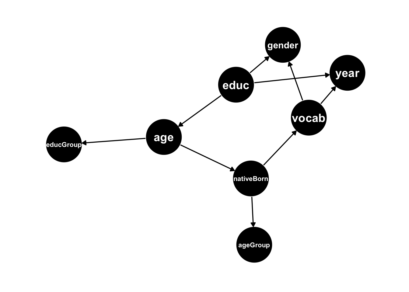
The DGP will be constructed using the non_parametric_dag_model function from simMixedDAG.
For every algorithm and sample size we simulate 200 datasets and measure the estimated DAG accuracy.
Below we can see the average simulation results for the edge distance measure for different samples sizes:
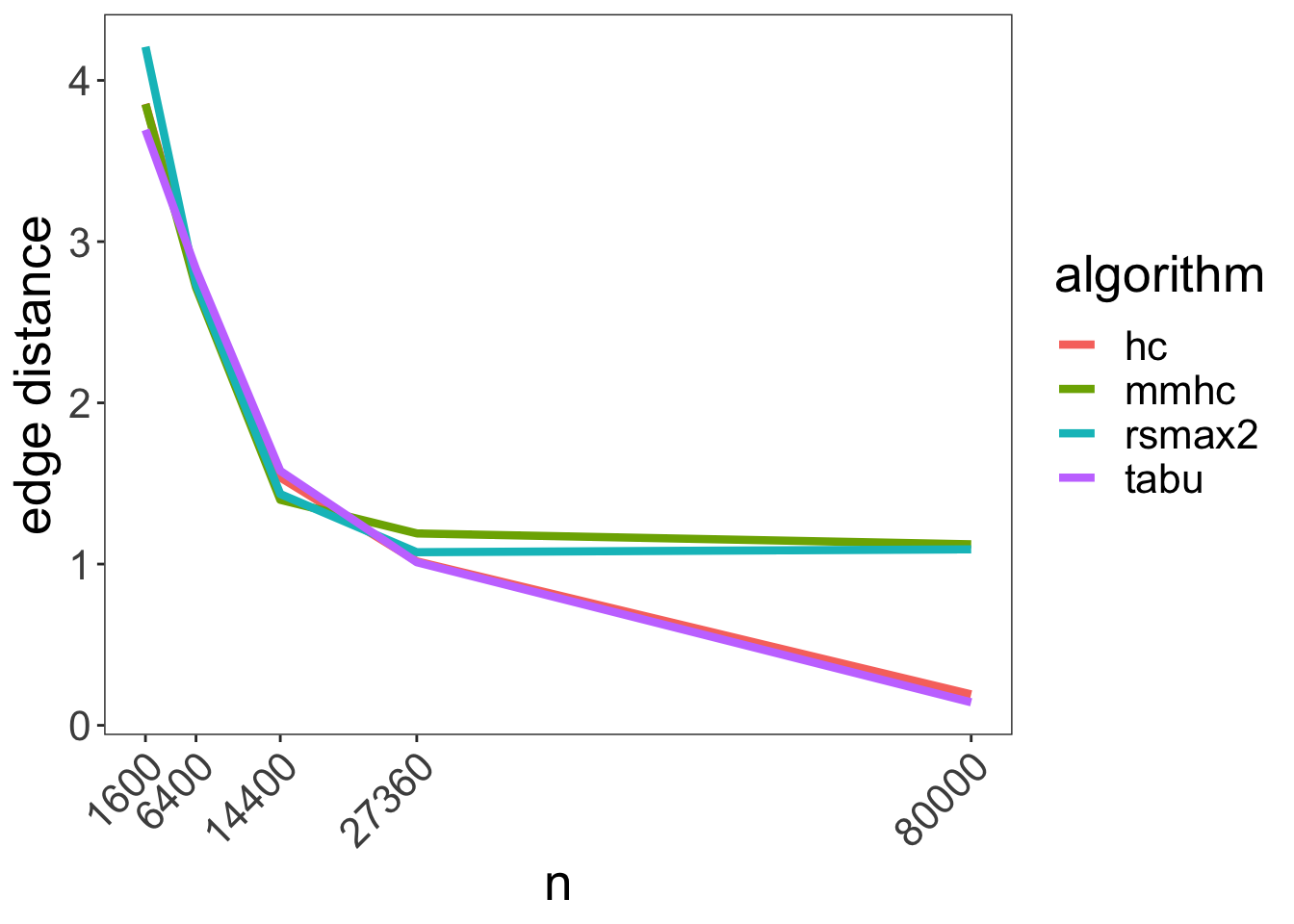
We can see that the algorithm performance is comparable up to around 27360 observations, after which mmhc and rsmax2 flatten out while hc and tabu approach perfect estimation of the DAG skeleton.
Below we can see the average simulation results for the Hamming distance measure:
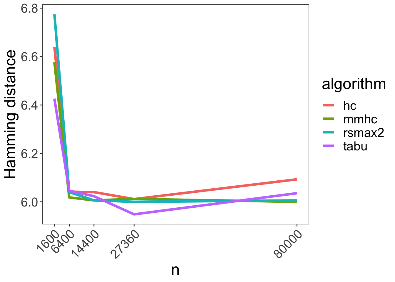
We can see that pretty fast all algorithms hit a performance plateau at around 6.
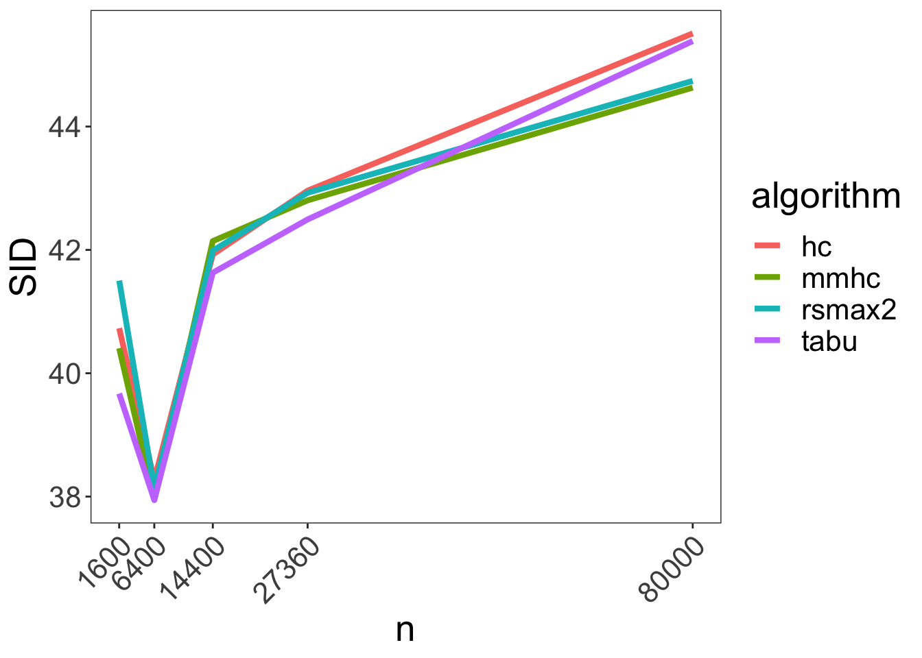
When it comes to Structural Intervention Distance things look even worse:
Let’s revisit that last one with error bars just for mmhc:
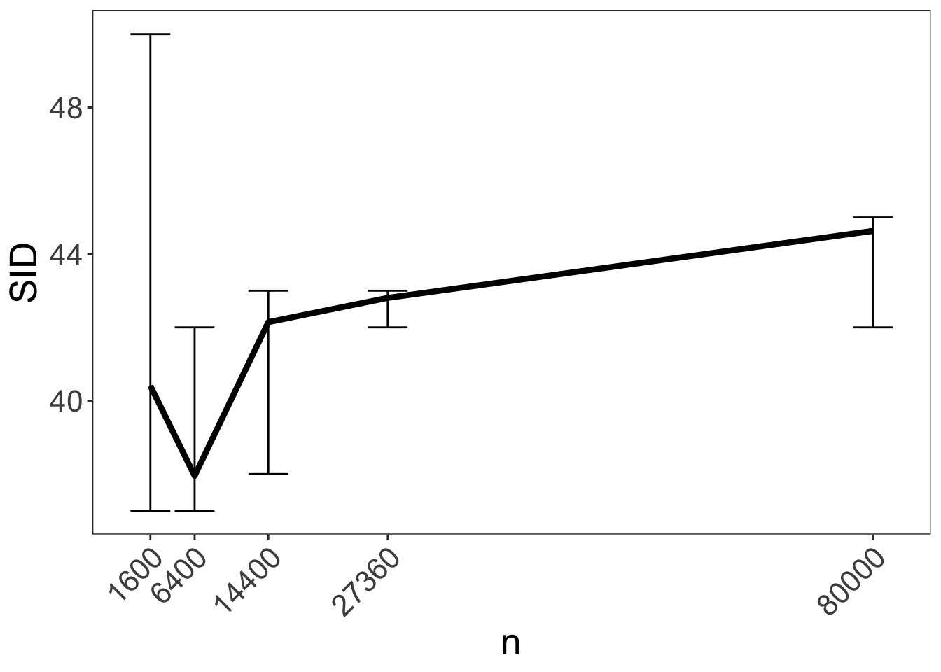
We can see that the performance is essentially unchanged across different sample sizes (all confidence intervals overlap).
To get a sense of what different SID scores mean, we can calculate the probability of finding the correct adjustment set given a random selection of a treatment and control pair using the following equation:
\[P(\text{correct adj set)} = 1 - \frac{SID}{\#\{\text{possible treatment - exposure pairs}\}}\] In our case given there are 8 nodes we have \(\#\{\text{possible treatment - exposure pairs}\} = 8 \cdot 7 = 56\).
Below is the resulting graph:
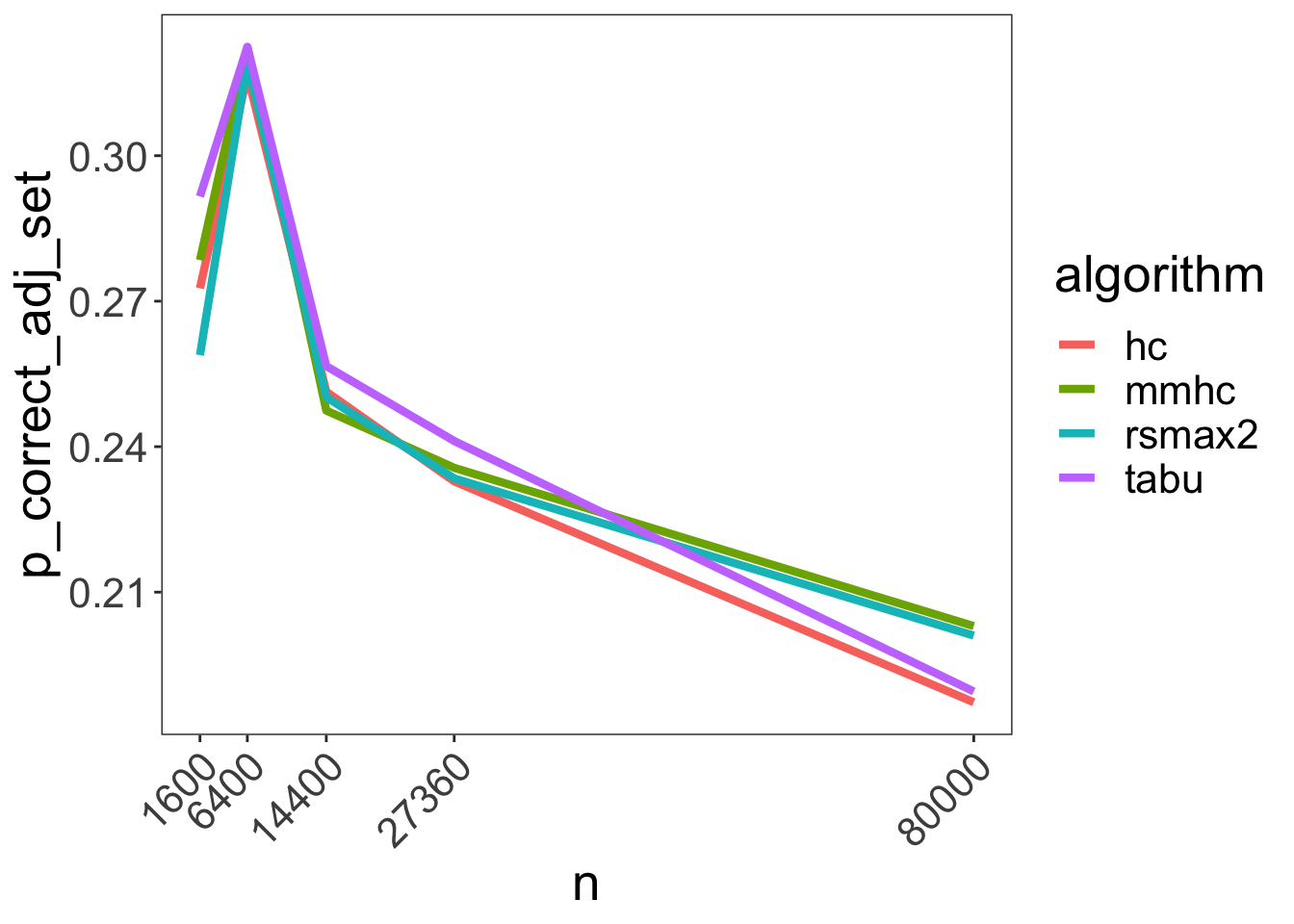
Pretty abysmal.
Summary
While all algorithms converge on the correct DAG skeleton as the sample size increases, none of them is able to orient the edges correctly. So at least for the algorithms surveyed, benchmarked on our specific simulated dataset it would seem automatic DAG learning isn’t a very reliable way to find the correct adjustment set.
All is lost?
Despair not! For in my next blog post I’ll introduce a small package I’ve written to address the issue of DAG edge orientation.