
Intro
I’ve discussed on several blog posts how Causal Inference involves making inference about unobserved quantities and distributions (e.g. we never observe \(Y|do(x)\)). That means we can’t benchmark different algorithms on Causal Inference tasks (e.g \(ATE/CATE\) estimation) the same way we do in ML because we don’t have any ground truth to benchmark against.
In the absence of ground truth, one of the main tools left for model comparison and performance bench-marking is simulation studies. On a recent post I used a semi synthetic dataset to benchmark different algorithms on the task of \(ATE/CATE\) estimation.
DAG estimation is another important task in Causal Inference on which I intend to write in a future post. The ground truth lacking in this case is the true DAG underlying a dataset. We thus need a way to simulate “realistic” datasets from known DAGs and compare how well different algorithms do at retrieving them.
When it comes to simulating data from DAGs there’s a slew of existing solutions in R. To name just a few:
- The
simulateSEMfunction from the “dagitty” package simulates continuous Gaussian variables only.
- The
dag.simfunction from the “dagR” package simulates continuous Gaussian and logit binary nodes (no multi level categorical). - The
rbnfunction from the “bnlearn” package can simulate mixed data type datasets (both Gaussian continuous and categorical) but categorical nodes can only have categorical parents.
All functions above generate datasets from parametric distributions, thus limiting how representative of “real” datasets the resulting simulations might be.
In an effort to enable better Causal Inference tasks bench-marking using “real life” datasets simulation I’ve written a small package: “simMixedDAG”.
In this post I’ll introduce the package and demonstrate it’s features.
You can install the “simMixedDAG” package from github. I like doing so using the great “pacman” package:
pacman::p_load_gh("IyarLin/simMixedDAG")Non parametric DAG simulation
When simulating data from a DAG, one has to specify for every node \(x_j\) some data generating process \(f_j\) which defines how the node is simulated from it’s parent nodes \(PA_j\). The DAG structure along with the functions \(f_j\) compose what I refere to as a “DAG model”.
Trying to specify non-parametric \(f_j\) can be pretty tedious (essentially drawing by hand the different marginal and joint distributions) and can also be not very realistic as not many of us have a good intuition as to how a “real life” non parametric distribution looks like.
What we can do instead is define the functions \(f_j\) as generalized additive models:
\[x_j = f_j(PA_j) = g\left(\sum_{i \in PA_j}s_{ij}(x_i) + \epsilon_j\right)\]
where \(g\) is a link function and \(s_{ij}(x_i)\) are smoothing functions.
Next, assuming some DAG we can fit the smoothing functions \(s_{ij}(x_i)\) from a real life dataset. The fitted functions can now be used to simulate new datasets. The resulting datasets have a known underlying DAG while maintaining marginal and joint distributions similar to those observed in a “real life” dataset.
Fitting and simulating a non paramateric DAG - an example
In this example we’ll use the General Social Survey dataset.
We’ll assume the following DAG for a subset of the variables:
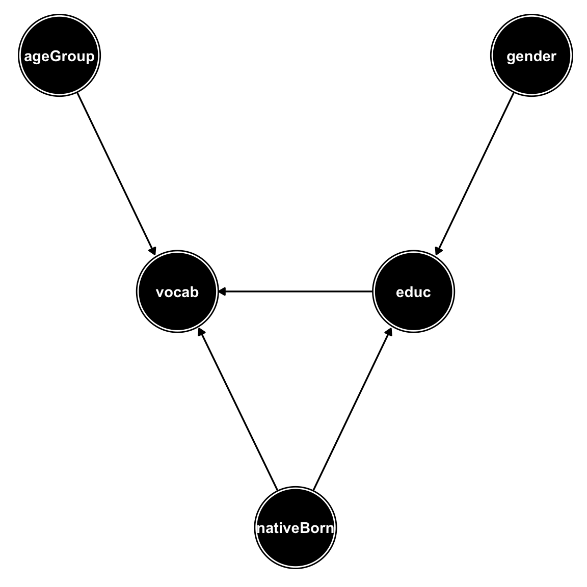
The following piece of code fits the smoothing functions \(s_{ij}(x_i)\) and stores them in an object of class “non_parametric_dag_model”:
non_param_dag_model <-
  non_parametric_dag_model(
    dag = g,
    data = GSSvocab
  )
Simulating new data from the dag_model object is simple as running:
sim_data <-
sim_mixed_dag(
dag_model = non_param_dag_model,
N = 30000
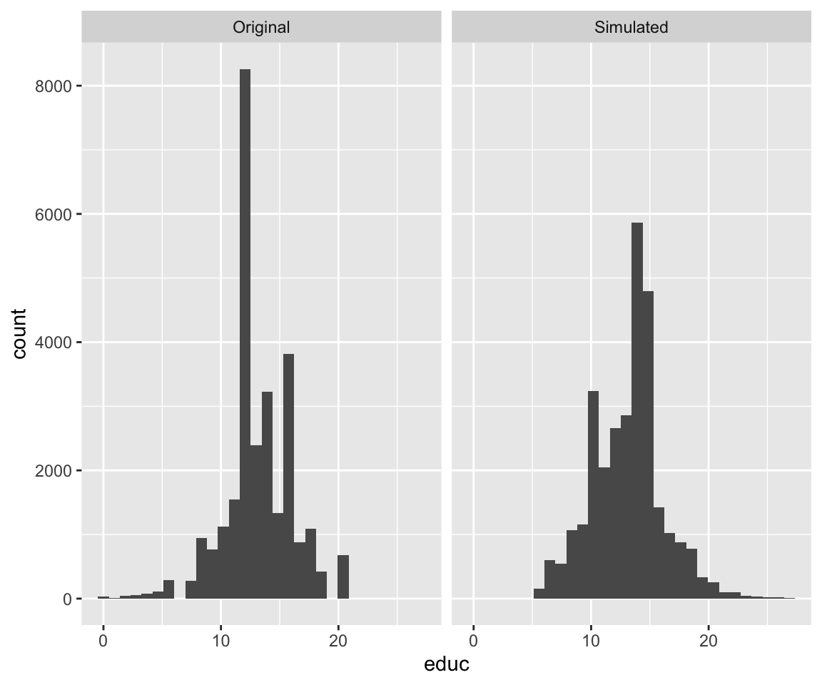
)We can verify that indeed the original distributions are mostly preserved in the simulated dataset:
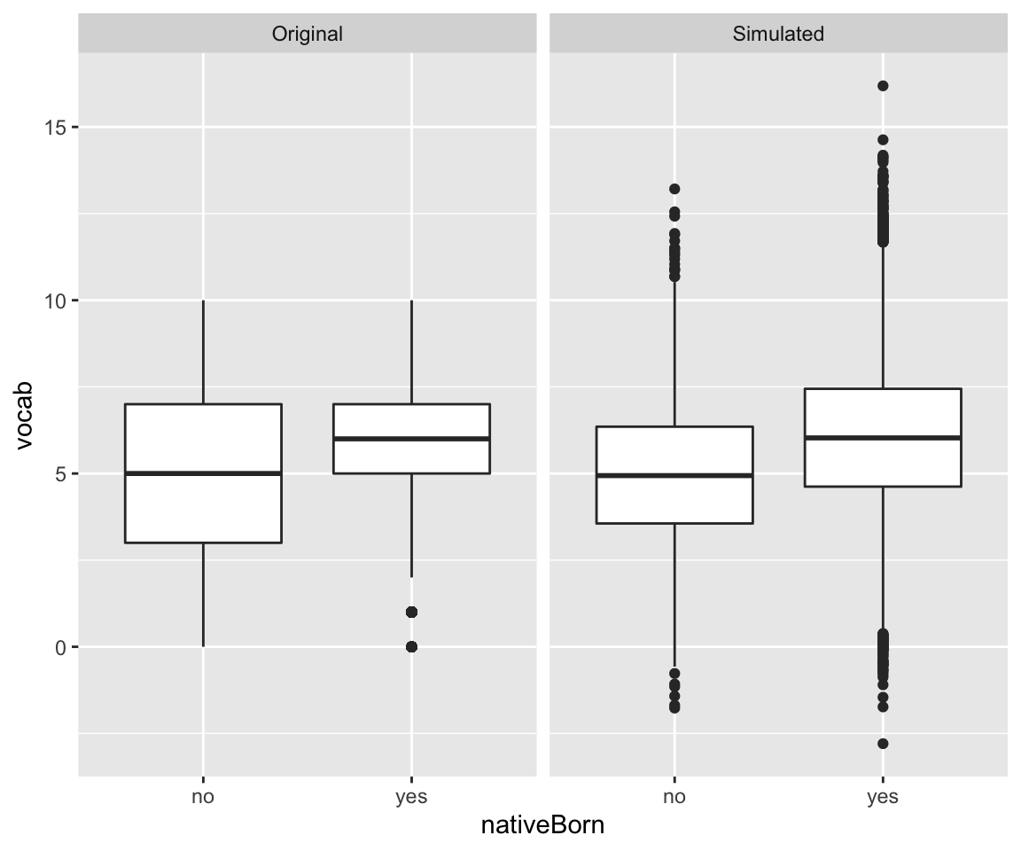
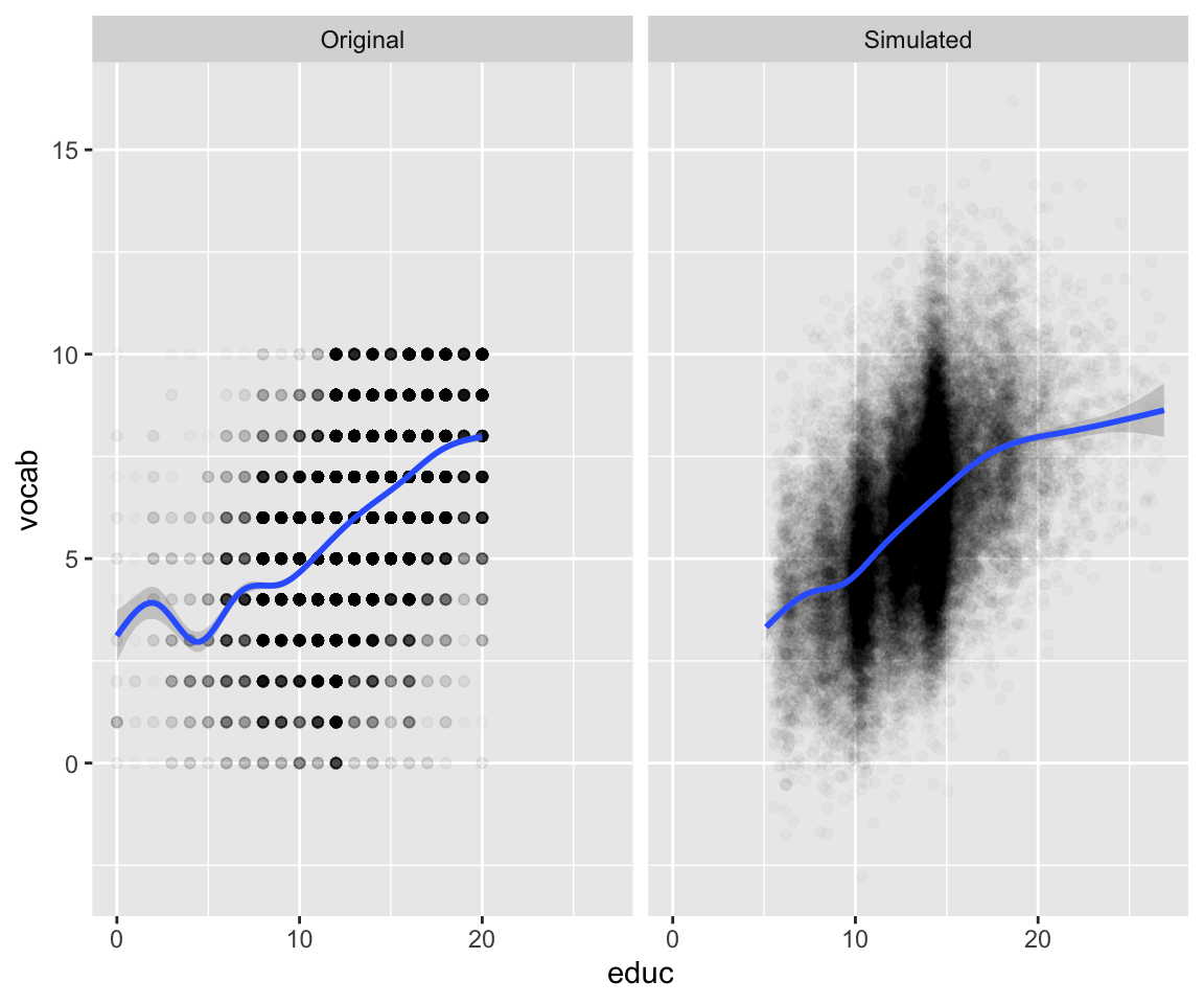
We notice vocab on the original dataset was constrained to the integers 0-10, while in the simulated dataset it was transformed to continuous with some values extending beyond the 0-10 range.
| nativeBorn | female | male |
|---|---|---|
| no | 0.0469 | 0.0387 |
| yes | 0.52 | 0.394 |
| nativeBorn | female | male |
|---|---|---|
| no | 0.0494 | 0.035 |
| yes | 0.52 | 0.395 |
Paramteric DAG simulation
The simMixedDAG provides functions for simulation of complex parametric DAG models as well. These can come handy when one wants to have more control over the specific functions \(f_j\). At it’s most basic form it can be used to simulate simple Gaussian nodes:
\[f_j(PA_j) = lp + \epsilon_j\] where \(lp\) is the linear combination of the node parents: \(lp = \sum_{i \in PA_j}\beta_{ij}x_i\).
Specifying and simulating a paramateric DAG - an example
In this example we’ll use the DAG presented on my first post:
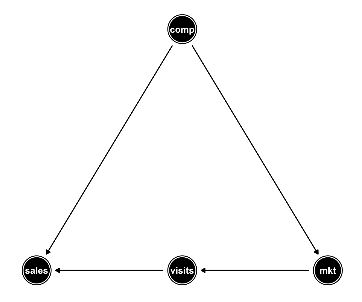
In the next few lines I specify a simple parametric DAG model with all Gaussian nodes and simulate a dataset from that model:
set.seed(2)
param_dag_model <- parametric_dag_model(dag = g)
sim_data <- sim_mixed_dag(dag_model = param_dag_model,
                          N = 500)
sim_data %>% ggplot(aes(comp, sales)) + geom_point() +
  stat_smooth(method = "lm")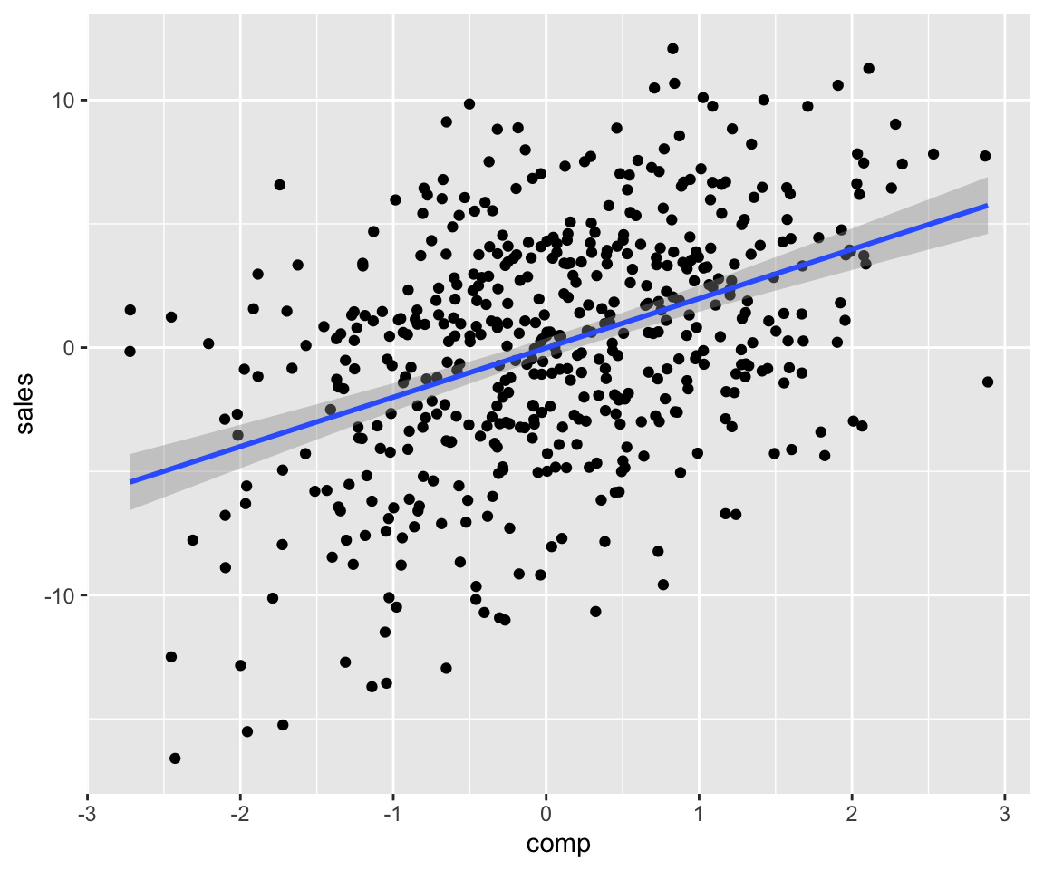
In the code above we didn’t specify what the \(\beta\) coefficients are. Those are thus drawn from a standard normal distribution.
We can manually set beta coefficients by providing an additional f.args argument as follows:
set.seed(1)
param_dag_model <-
  parametric_dag_model(
    dag = g, f.args =
      list(sales = list(betas = list(comp = -2)))
  )
sim_data <- sim_mixed_dag(param_dag_model, N = 500)
sim_data %>% ggplot(aes(comp, sales)) + geom_point() +
  stat_smooth(method = "lm")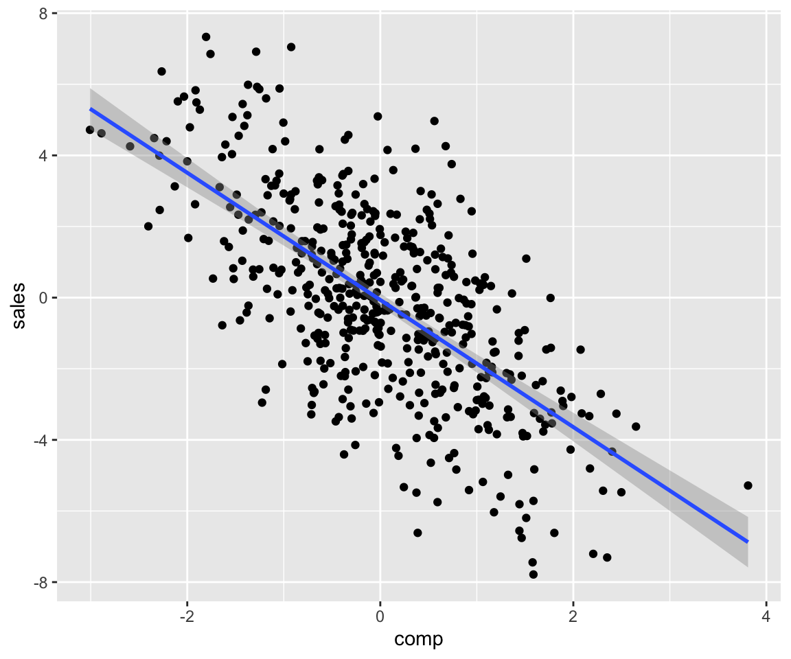
We can set how noisy the errors are using the sinr (signal to noise ratio) argument:
set.seed(1)
param_dag_model <-
  parametric_dag_model(dag = g, f.args = list(
    sales = list(betas = list(comp = -2), sinr = 5),
    mkt = list(betas = list(comp = 0))
  ))

sim_data <- sim_mixed_dag(param_dag_model)

sim_data %>% ggplot(aes(comp, sales)) + geom_point() +
  stat_smooth(method = "lm")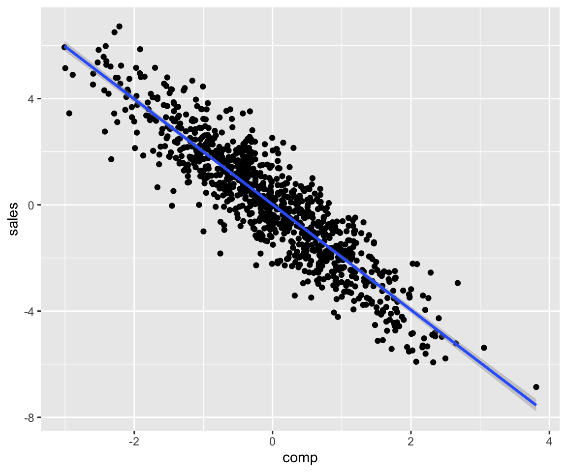
We can tweak the \(f\) functions to include a link function \(g\):
\[f_j(PA_j) = g(lp) + \epsilon_j\]
Below I apply a “cosin” link function using the link argument:
set.seed(1)
param_dag_model <-
  parametric_dag_model(dag = g, f.args = list(
    sales = list(betas = list(comp = -2),
                 link = "cosin",
                 sinr = 3),
    mkt = list(betas = list(comp = 0))
  ))

sim_data <- sim_mixed_dag(param_dag_model)

sim_data %>% ggplot(aes(comp, sales)) + geom_point() +
  stat_smooth()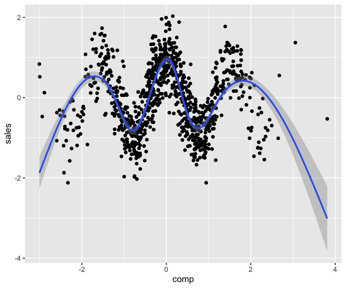
Below are 2 more link functions implemented:
set.seed(1)
param_dag_model <-
  parametric_dag_model(dag = g, f.args = list(
    sales = list(betas = list(comp = -2),
                 link = "quadratic",
                 sinr = 3),
    mkt = list(betas = list(comp = 0))
  ))

sim_data <- sim_mixed_dag(param_dag_model)

p1 <- sim_data %>% ggplot(aes(comp, sales)) +
  geom_point() + stat_smooth() +
  ggtitle("Quadratic") +
  theme(plot.title = element_text(hjust = 0.5))

param_dag_model <-
  parametric_dag_model(dag = g, f.args = list(
    sales = list(betas = list(comp = -2),
                 link = "exp",
                 sinr = 3),
    mkt = list(betas = list(comp = 0))
  ))

sim_data <- sim_mixed_dag(param_dag_model)

p2 <- sim_data %>% ggplot(aes(comp, sales)) +
  geom_point() + stat_smooth() +
  ggtitle("Exponent") +
  theme(plot.title = element_text(hjust = 0.5))

grid.arrange(p1, p2, nrow = 1)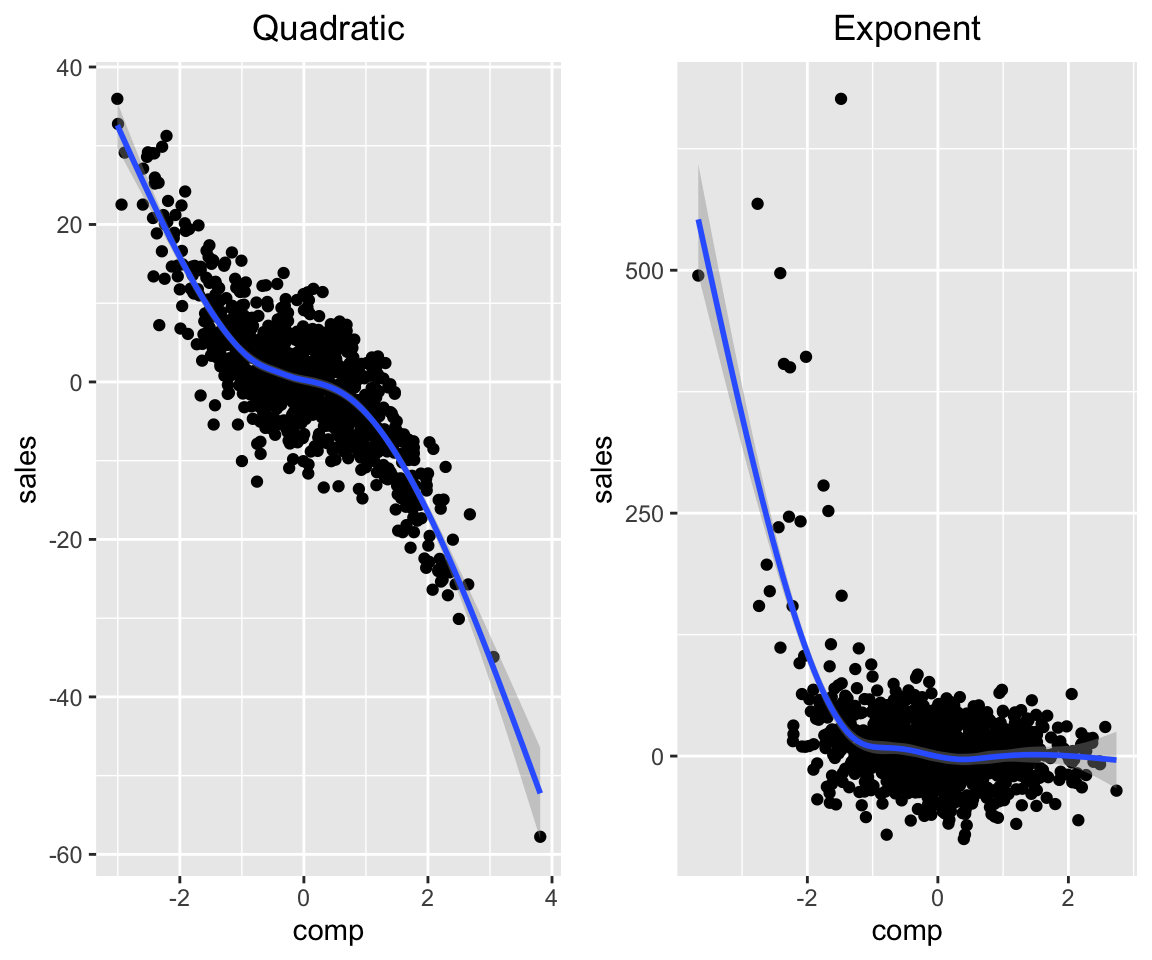
We introduce categorical variables with \(M\) levels via the following transformation:
\[f_j(PA_j) = cat(g(lp) + \epsilon_j)\] where we have:
\[ cat(x) = \begin{cases} \text{level 1,} &\quad\text{if} \, x \leq \Phi^{-1}(100/M) \\ \text{level 2,} &\quad\text{if} \, x > \Phi^{-1}(100/M) \, , x/sd(x) \leq \Phi^{-1}(100\cdot 2/M)\\ \dots & \dots \\ \text{level M,} &\quad\text{if} \, x > \Phi^{-1}(100\cdot(M-1)/M) \\ \end{cases} \]
We set the number of levels using the levels argument (where levels = 1 means continuous variable):
param_dag_model <-
  parametric_dag_model(dag = g,
      f.args = list(sales = list(
    betas = list(comp = -2),
    link = "quadratic", sinr = 3, levels = 3,
    labels = c("low", "medium", "high")
  ), mkt = list(betas = list(comp = 0))))

sim_data <- sim_mixed_dag(param_dag_model)

sim_data %>% ggplot(aes(sales, comp)) + geom_boxplot() +
  stat_smooth()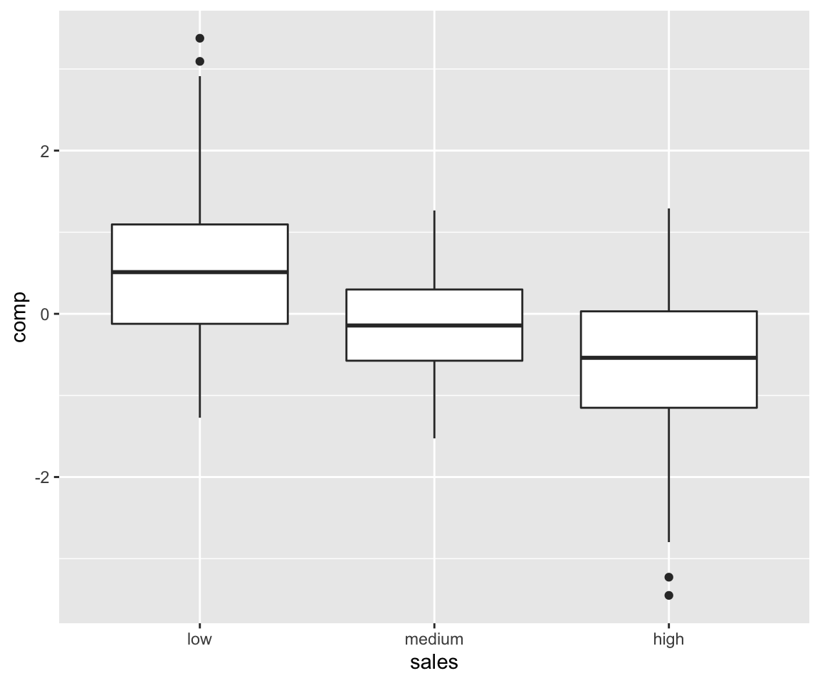
It’s important to note that any non-specified arguments in f.args are filled in from default values.
Calculating ATE given a DAG model
The “simMixedDAG” package can be used for bench-marking algorithms on the task of \(ATE\) estimation.
For simple DAG models the analytic calculation of the \(ATE\) is pretty simple (e.g. continuous Gaussian distributed, no interactions etc). When simulating from more complex models (e.g. parametric with link functions, non parametric models) deriving the ATE analytically might become more challenging.
One way to obtain the true \(ATE\) given a DAG model is to use simulation analysis. Consider for instance the problem setup discussed on my first post where we calculated analytically that the \(ATE\) of mkt on sales was 0.15.
We know that the relation of \(mkt\) to \(sales\) is confounded by the \(comp\) variable. When setting \(mkt\) to some value (AKA \(do(mkt)\)) we remove the arrow that points from \(comp\) to \(mkt\) (like in the DAG below):
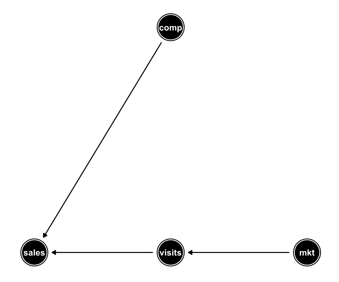
The above operation of removing all arrows pointing into the treatment variable is also called “graph surgery” (See Pearl’s “Causal Inference in Statistics - A Primer” chapter 3).
When observing the by-variate relation in the non-confounded dataset simulated from the DAG above we can see the true effect of \(mkt\) on \(sales\):
param_dag_model <-
  parametric_dag_model(dag = g_unconfounded,
                       f.args = list(
    sales = list(betas = list(visits = 0.3,
                              comp = -0.9)),
    visits = list(betas = list(mkt = 0.5))
  )) # note here we set the comp to mkt
     # coefficient to 0
sim_data <- sim_mixed_dag(param_dag_model)
sim_data %>% ggplot(aes(mkt, sales)) + geom_point() +
  stat_smooth(method = "lm")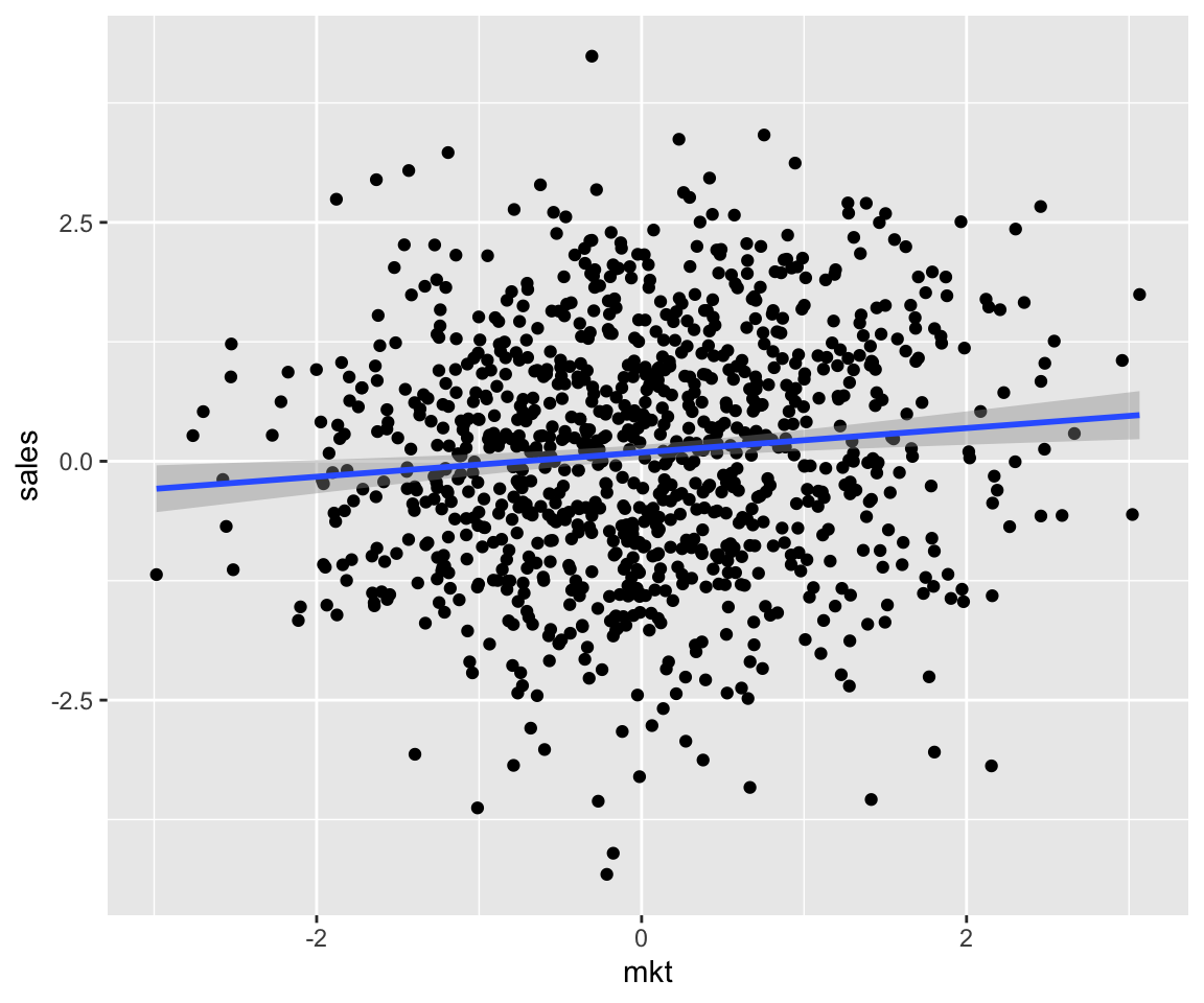
The get_ate function implements the same logic under the hood to calculate the \(ATE\) for any dag_model. Below we demonstrate using the following code:
param_dag_model <-
  parametric_dag_model(dag = g, f.args = list(
    sales = list(betas = list(visits = 0.3,
                              comp = -0.9)),
    visits = list(betas = list(mkt = 0.5)),
    mkt = list(betas = list(comp = 0.6))
  )) # note the comp to mkt coefficient is as
     # in the original probelm setup

mkt_ATE_on_sales <- get_ate(param_dag_model,
  treatment = "mkt",
  treatment_vals = -2:2, exposure = "sales"
)
pandoc.table(mkt_ATE_on_sales,
caption = "mkt ATE on sales")| from | to | ATE |
|---|---|---|
| -2 | -1 | 0.1514 |
| -1 | 0 | 0.1482 |
| 0 | 1 | 0.1502 |
| 1 | 2 | 0.1512 |
We can verify that indeed we got the outcome derived analytically.
Now let’s take a more complicated model defined by the following equations:
\[sales = quadratic\left(1.5 \cdot visits -4 \cdot comp\right) + \epsilon_{sales}\]
\[visits = 0.5I(mkt = "medium") + 1.2I(mkt = "high") + \epsilon_{visits}\]
\[mkt = cat(exp(2 \cdot comp) + \epsilon_{mkt})\] with \(mkt\) taking the levels “low”, “medium” and “high”.
Below is the code to define the model defined by the equations above and get the corresponding ate of mkt on sales.
param_dag_model <- parametric_dag_model(dag = g,
                                        f.args = list(
    sales = list(betas = list(visits = 1.5, comp = -4),
                 link = "quadratic"),
    visits = list(betas = list(mkt = c(0.5, 1.2)),
                  levels = 1),
    mkt = list(
      betas = list(comp = 2), levels = 3,
      labels = c("low", "medium", "high"),
      link = "exp", sinr = 8
    )
  ))

treat_vals <- factor(c("low", "medium", "high"),
                  levels = c("low", "medium", "high"))
mkt_ate_on_sales <-
  get_ate(param_dag_model, treatment = "mkt",
          treatment_vals = treat_vals,
          exposure = "sales")

pandoc.table(mkt_ate_on_sales,
caption = "mkt ATE on sales")| from | to | ATE |
|---|---|---|
| low | medium | 5.139 |
| medium | high | 7.518 |
Below we verify we got the correct result by simulating the unconfounded dataset and measuring the difference between average sales for by mkt:
param_dag_model$f.args$mkt$betas$comp <- 0
sim_data <- sim_mixed_dag(param_dag_model, N = 1000000)
sim_data %>%
  group_by(mkt) %>%
  summarise(sales = mean(sales)) %>%
  mutate(sales_diff = sales - lag(sales)) %>%
pandoc.table()| mkt | sales | sales_diff |
|---|---|---|
| low | 0.147 | NA |
| medium | 4.82 | 4.673 |
| high | 11.97 | 7.149 |
Seems close enough.
Let’s go back to the non-parametric model we defined earlier and calculate the \(ATE\) of educ on vocab:
educ_ate_on_vocab <-
  get_ate(non_param_dag_model,
    treatment = "educ",
    exposure = "vocab",
    treatment_vals = c(0, 12, 15, 17, 20),
    M = 300
  ) %>%
  mutate(min_education = c("high school",
                           "1st degree",
                           "2nd degree",
                           "PhD"))
pandoc.table(educ_ate_on_vocab,
caption = "educ ATE on vocab")| from | to | ATE | min_education |
|---|---|---|---|
| 0 | 12 | 2.228 | high school |
| 12 | 15 | 1.119 | 1st degree |
| 15 | 17 | 0.7399 | 2nd degree |
| 17 | 20 | 0.5299 | PhD |
It would seem academic accomplishments have diminishing returns.
An acknowledgement
Kudos to Guangchuang YU for authoring the cool hexSticker package, which makes creating hexagon sticker for your package (like the one at the top of this post) a breeze.