Machine learning applications have been growing in volume and scope rapidly over the last few years. What’s Causal inference, how is it different than plain good ole’ ML and when should you consider using it? In this post I try giving a short and concrete answer by using an example.

A typical data science task

Imagine we’re tasked by the marketing team to find the effect of raising marketing spend on sales. We have at our disposal records of marketing spend (mkt), visits to our website (visits), sales, and competition index (comp).

We’ll simulate a dataset using a set of equations (also called structural equations):

\[\begin{equation} sales = \beta_1vists + \beta_2comp + \epsilon_1 \end{equation}\] \[\begin{equation} vists = \beta_3mkt + \epsilon_2 \end{equation}\] \[\begin{equation} mkt = \beta_4comp + \epsilon_3 \end{equation}\] \[\begin{equation} comp = \epsilon_4 \end{equation}\]

with \(\{\beta_1, \beta_2, \beta_3\, \beta_4\} = \{0.3, -0.9, 0.5, 0.6\}\)

All data presented in graphs or used to fit models below is simulated from the above equations.

Below are the first few rows of the dataset:

mkt	visits	sales	comp
282.5	2977	379	3.635
338.8	3149	308	4.515
303.9	2485	369	3.092
558.8	3117	191	5.22
334.4	4038	286	4.281
297.7	2854	441	3.592

Our goal is to predict the effect of raising marketing spend on sales which is 0.15 (from the set of equations above, using product decomposition we get \(\beta_1 \cdot \beta_3 = 0.3 \cdot 0.5 = 0.15\)).

Common analysis approaches

First approach: plot bi-variate relationship

Many of us would start off by plotting a scatter plot of sales by marketing:

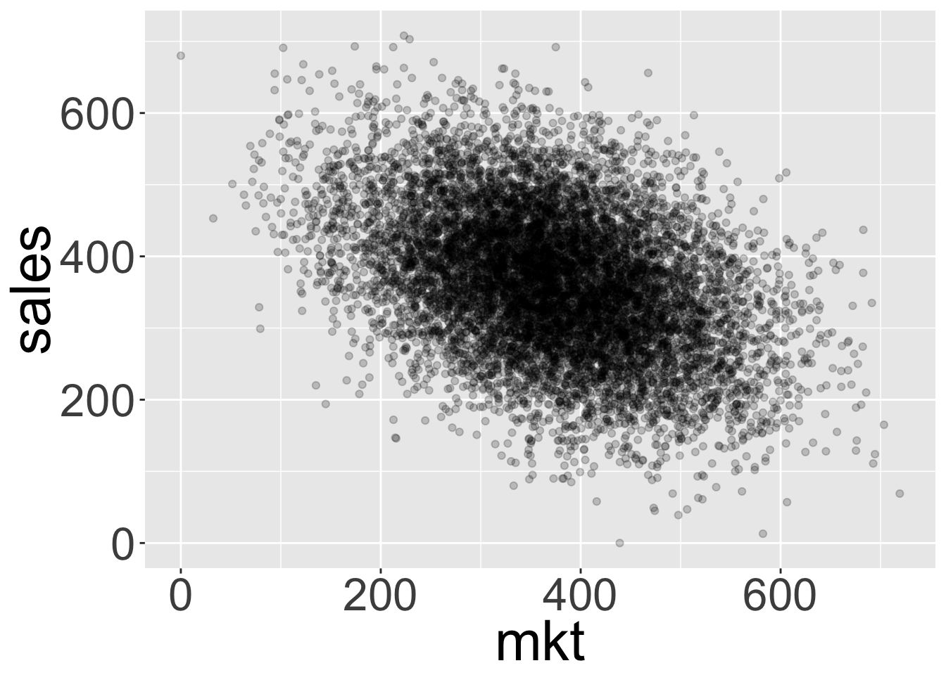
We can see that the relationship seen in the graph is actually the opposite of what we’d expected! It looks like increasing marketing actually decreases sales. Indeed, not only correlation isn’t causation, at times it can show a relation opposite to the true causation.

Fitting a simple linear model \(sales = r_0 + r_1mkt + \epsilon\) would yield the following coefficients: (note \(r\) is a regression coefficient where’s \(\beta\) is a true parameter in the structural equations)

(Intercept)	mkt
513.5	-0.3976

Confirming that we get a vastly different effect than the one we were looking for (0.15).

Second approach: Use ML model with all available features

One might postulate that looking on a bi-variate relation amounts to using only 1 predictor variable, but if we were to use all of the available features we might be able to find a more accurate estimate.

When running the regression \(sales = r_0 + r_1mkt + r_2visits + r_3comp + \epsilon\) we get the following coefficients:

(Intercept)	mkt	visits	comp
596.7	0.009642	0.02849	-90.06

Now it looks like marketing spend has almost no effect at all! Since we simulated the data from a set of linear equations we know that using more sophisticated models (e.g. XGBoost, GAMs) can’t produce better results (I encourage the skeptic reader to try this out by re-running the Rmd script used to produce this report).

Maybe we should consider the relation between features too…

Quite baffled by the results obtained so far we turn to consult the marketing team and we learn that in highly competitive markets the team would usually increase marketing spend (this is reflected in the coefficient \(\beta_4 = 0.6\) above). So it’s possible that competition is a “confounding” factor: when we observe high marketing spend there’s also high competition thus leading to lower sales.

Also, we notice that marketing probably affects visits to our site and those visits in turn affect sales.

We can visualize these feature inter-dependencies with a directed a-cyclic graph (DAG):

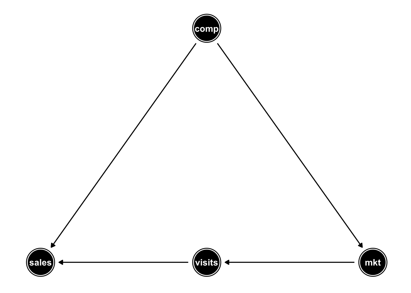
So it would make sense to account for the confounding competition by adding it to our regression. Adding visits to our model however somehow “blocks” or “absorbs” the effect of marketing on sales so we should omit it from our model.

Fitting the model \(sales = r_0 + r_1mkt + r_2comp + \epsilon\) yields the coefficients below:

(Intercept)	mkt	comp
654.8	0.1494	-89.8

Now we finally got the right effect estimate!

The way we got there was a bit shaky though. We came up with general concepts such as “confounding” and “blocking” of features. Trying to apply these to datasets consisting of tens of variables with complicated relationships would probably prove tremendously hard.

So now what? Causal inference!

So far we’ve seen that trying to estimate the effect of marketing spend on sales by examining bi-variate plots can fail bad. We’ve also seen that standard ML practices of throwing all available features into our model can fail too. It would seem we need to carefully construct the set of covariates included in our model in order to obtain the true effect.

In causal inference this covariate set is also termed “adjustment set”. Given a model DAG we can utilize various algorithms that rely on rules very much like those mentioned above such as “confounding” and “blocking”, to find the correct adjustment set.

Backdoor criteria

One of the most basic algorithms that can obtain the correct adjustment set is the “Backdoor-criteria” developed by J. Pearl. In a nutshell it seeks adjustment sets that block every “spurious” paths between our “exposure” variable (e.g. marketing) and “outcome” variable (e.g. sales) while keeping directed baths open.

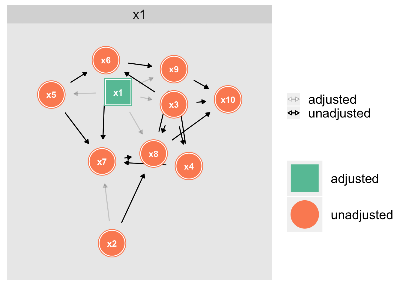
Consider for example the DAG below where we’re interested in finding the effect of x5 on x10:

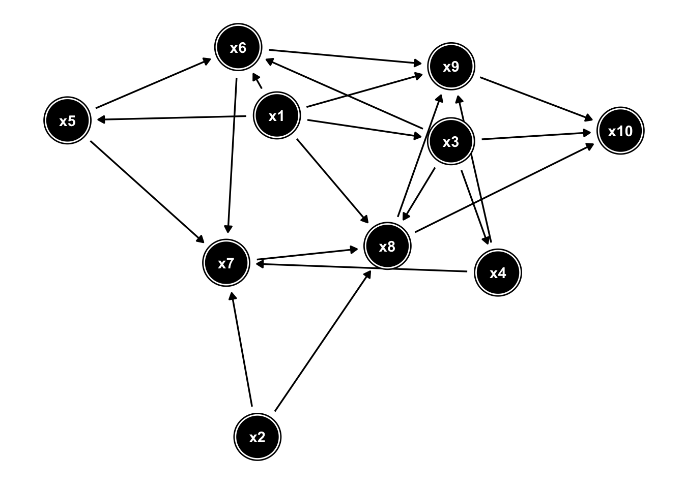
Using the backdoor-criterion (implemented in the R package “dagitty”) we can find the correct adjustment set:

How to obtain model DAGs?

Finding the model DAG can be admittedly challenging. It can be done using any combination of the following:

Use domain knowledge
Given a few candidate model DAGs one can perform statistical tests to compare their fit to the data at hand
Use search algorithms (e.g. those implemented in the R “mgm” or “bnlearn” packages)

I’ll touch upon this subject in more breadth in a future post.

"Correlation does not imply causation". So what does?