
Intro
On my last few posts I’ve tried answering high level questions such as “What is Causal inference?”, “How is it different than ML?” and “When should I use it?”.
In this post we finally get our hands dirty with some Kaggle style Causal Inference algorithms bake off! In this competition I’ll pit some well known ML algorithms vs a few specialized Causal Inference (CI) algorithms and find out who’s hot and who’s not!
Causal Inference objectives and the need for specialized algorithms
ATE: Average Treatment Effect
So far we’ve learned that in order to estimate the causal dependence of \(Y\) on \(X\) we need to use a set of features \(Z_B\) that satisfies the “Backdoor criteria”. We can then use the g-computation formula:
\[\mathbb{E}(Y|do(x)) = \sum_{z_B}f(x,z_B)P(z_B)\]
where \(Y\) is our target variable, \(do(x)\) is the action of setting a treatment \(X\) to a value \(x\) (see my previuos post for more details on the do operator) and \(f(x,z_B) = \hat{\mathbb{E}}(Y|x,z_B)\) is some predictor function we can obtain using regular ML algorithms.
One might ask: if we can obtain \(f(x,z_B)\) using regular ML algorithms why the need for specialized CI algorithms?
The answer is that our objective in CI is different than our objective in classic ML: In ML we seek to predict the absolute value of Y given we observed \(X\) take value \(x\): \(\mathbb{E}(Y|x)\), while in CI we try to estimate the difference in the expected value of \(Y\) across different assignment values \(x\) of \(X\). In the CI literature this quantity is termed “Average Treatment Effect” or in short \(ATE\). In the binary treatment case (where \(X \in \{0, 1\}\)) it’s defined as:
\[ATE := \mathbb{E}(Y|do(1)) -\mathbb{E}(Y|do(0))\]
and in the general (not necessarily binary treatment) case it’s defined as:
\[ATE(x) := \frac{\partial \, \mathbb{E}(Y|do(x))}{\partial \, x}\]
To see why accurate estimation of \(\mathbb{E}(Y|x)\) doesn’t necessarily mean accurate estimation of the \(ATE\) (and thus different objectives might require different algorithms) let’s look at an example:
Imagine we work for a company in the marketing industry. The treatment in this example is an automatic AI bidding robot we’ve developed recently as a value added service for our campaigns management platform. In order to demonstrate it works we sold it in a trial version for a few months, at the end of which we recorded for all our customers whether they took the trial (“treated”) or not (“untreated”), average campaign ROI and company size (“small” or “large”):
| treatment | company size | ROI | Proportion |
|---|---|---|---|
| untreated | small | 1% | 0.1 |
| treated | small | 2% | 0.4 |
| untreated | large | 5% | 0.4 |
| treated | large | 5% | 0.1 |
The first line reads “The average ROI for campaigns run by small companies who didn’t use our robot (untreated) is 1%. The proportion of those campaigns of the entire campaigns run on our platform is 0.1.
In order to use the g-computation formula we need to identify the correct adjustment set \(Z_B\).
After talking to some of our customers we learn that large companies usually employ large teams of analysts to optimize their campaigns, resulting in higher ROI compared with smaller companies. Having those large teams also means they have lower tendency to run our trial compared with small companies.
We thus assume the following DAG:
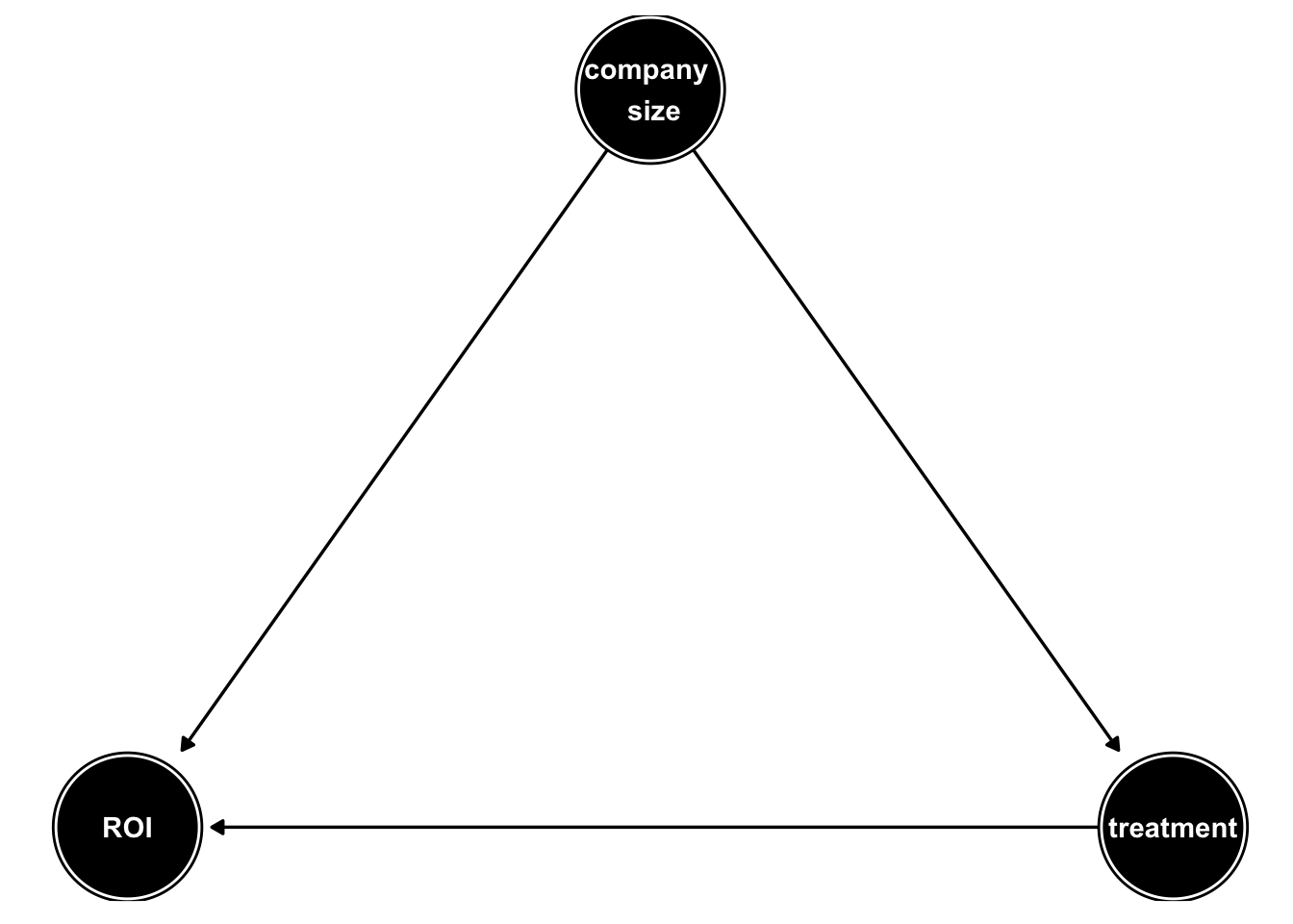
Applying the “Backdoor criteria” to the DAG above we arrive at the insight that company size is a confounding factor and thus \(Z_B = \text{company size}\). The g-computation formula reads in our case:
\[\begin{equation} \mathbb{E}(\text{ROI}|do(\text{treatment})) = \\ \sum_{\text{company size} \in \{\text{small, large}\}}\mathbb{E}(\text{ROI}|\text{treatment, company size})P(\text{company size}) \end{equation}\]We thus arrive at the quantities:
\[\mathbb{E}(\text{ROI}|do(\text{treated})) = \\ 2\% \cdot (0.4 + 0.1) + 5\% \cdot (0.1 + 0.4) = 3.5\%\]
and
\[\mathbb{E}(\text{ROI}|do(\text{untreated})) = \\ 1\% \cdot (0.4 + 0.1) + 5\% \cdot (0.1 + 0.4) = 3\%\]
and finally
\[ATE = \mathbb{E}(\text{ROI}|do(\text{treated})) - \mathbb{E}(\text{ROI}|do(\text{untreated})) = 0.5\%\]
Meaning the treatment (our robot) increases ROI by 0.5% on average.
Next, let’s assume our data is noisy and the average ROI isn’t enough to estimate the expected ROI. We try to estimate the ROI using 2 models. Below we can see the model predictions (with absolute error in parenthesis):
| treat | comp size | Prop | ROI (true, unknown) | ROI (model 1) | ROI (model 2) |
|---|---|---|---|---|---|
| untreated | small | 0.1 | 1% | 1.5% (0.5%) | 0% (1%) |
| treated | small | 0.4 | 2% | 1.5% (0.5%) | 1% (1%) |
| untreated | large | 0.4 | 5% | 5.5% (0.5%) | 4% (1%) |
| treated | large | 0.1 | 5% | 4.5% (0.5%) | 4% (1%) |
We can see that model 1 is more accurate than model 2 in every row.
If we were to use model 1 to estimate the \(ATE\) we’d get:
\[\hat{\mathbb{E}}(\text{ROI}|do(\text{treated}))_{\text{mode1}} = \\ 1.5\% \cdot (0.4 + 0.1) + 4.5\% \cdot (0.1 + 0.4) = 3\%\]
and
\[\hat{\mathbb{E}}(\text{ROI}|do(\text{untreated}))_{\text{mode1}} = \\ 1.5\% \cdot (0.4 + 0.1) + 5.5\% \cdot (0.1 + 0.4) = 3.5\%\]
and finally
\[\hat{ATE}_{\text{mode1}} = -0.5\%\]
Meaning we estimate our product to decreases ROI by 0.5%! Our estimate is not only wrong in magnitude but also in sign, meaning we can’t use it to market our product.
If we were to use model 2 however we’d get:
\[\hat{\mathbb{E}}(\text{ROI}|do(\text{treated}))_{\text{model2}} = \\ 1\% \cdot (0.4 + 0.1) + 4\% \cdot (0.1 + 0.4) = 2.5\%\]
and
\[\hat{\mathbb{E}}(\text{ROI}|do(\text{untreated}))_{\text{model2}} = \\ 0\% \cdot (0.4 + 0.1) + 4\% \cdot (0.1 + 0.4) = 2\%\]
and finally
\[\hat{ATE}_{\text{model2}} = 0.5\%\]
Arriving at the correct \(ATE\) estimate! So even though model 2 is less accurate than model 1 in estimating \(\mathbb{E}(\text{ROI})\), it’s better in estimating the \(ATE\).
CATE: Conditional Average Treatment Effect
Looking at the table above we see that while our product increases ROI by 0.5% on average, it increases ROI by 1% for campaigns run by small companies, while not improving at all those run by large ones. We’ll be thus well advised to market our product to small companies.
In the CI literature the treatment effect conditioned on some other features \(z\) (such as company size) is fittingly termed “Conditional Average Treatment Effect” (\(CATE\)). In cases where the features conditioned on identify individuals uniquely (e.g. when at least one of the features conditioned on is continuous) it is also termed “Individual Treatment Effect”, which is a highly sought after quantity in personalized medicine for example. For the binary case the \(CATE\) is defined as:
\[CATE(z) := \mathbb{E}(Y|do(1),z) - \mathbb{E}(Y|do(0),z)\]
In the general (not necessarily binary treatment) case it’s defined as:
\[CATE(x, z) := \frac{\partial \, \mathbb{E}(Y|do(X=x), Z=z)}{\partial \, x}\]
Looking again at the model predictions above we can compare the actual vs predicted \(CATE\) for both models (with absolute error in parentheses):
| comapny size | CATE (true, unknown) | CATE (model 1) | CATE (model 2) |
|---|---|---|---|
| small | 1% | 0% (1%) | 1% (0%) |
| large | 0% | -1% (1%) | 0% (0%) |
Again, we can see that while model 1 was more accurate than model 2 in predicting \(\mathbb{E}(Y)\), it entirely misses the true \(CATE\) while model 2 estimates it perfectly.
To summarize: Specialized CI algorithms might be necessary because different objectives might require different tools.
An example with simulated data
The example above might seem a bit ad hoc (which is true) but it is motivated by possibly real scenarios. I’ll demonstrate by simulating a small (100 observations) dataset from the example problem presented above and fit to it a simple decision tree. Below is the resulting tree:
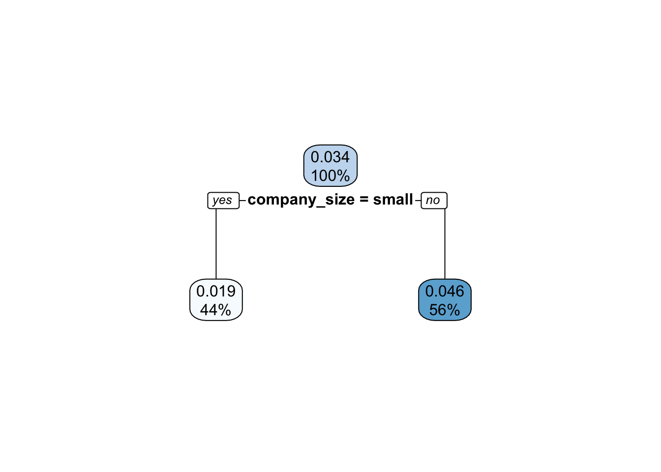
We can see that the tree completely ignored the treatment! To see why that happened let’s take a look at the dataset distribution:
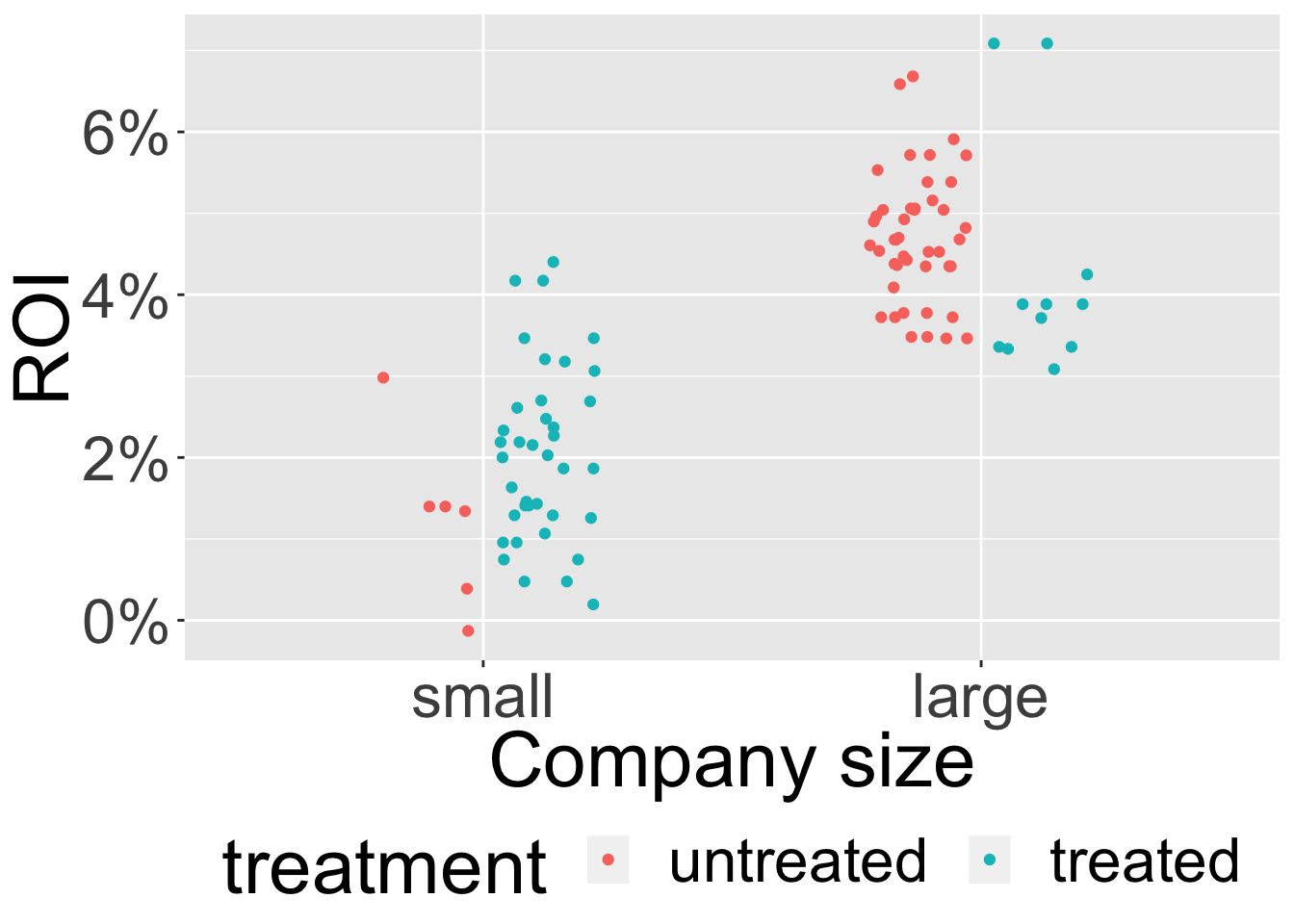
We can see in the graph above 2 dataset features that could potentially throw off regular ML algorithms when in comes to CI tasks:
- The variability due to the treatment is very small compared with that of other features in the dataset leading to an underestimate of the treatment effect (In the graph the variability due to company size is much higher than that of the treatment, which is why the decision tree disregarded the treatment).
- The distribution of features among the treatment groups is highly skewed (in the graph we can see the treated units make up the vast majority in the small companies and a small minority in the large companies, making the comparison within each company size unreliable and thus estimating the \(CATE\) very hard).
In the showdown below we’ll see if more powerful ML algorithms can still hold their own against algorithms designed specifically for CI tasks.
The competition setup
It’s now time to setup the problem for our competition!
In this competition I’ll use a semi-synthetic dataset generated for the “Atlantic Causal Inference Conference” Data Analysis Challenge. The “real data” part comprises of the feature set \(Z\), which contains 58 measurements taken from the Infant Health and Development Program. Those include features such as mother’s age, endocrine condition, child’s bilirubin etc.
Of the full feature set \(Z\) only a subset of 8 features consists the correct adjustment set \(Z_B\) while the rest are nuisance (meaning they do not affect the treatment nor the target variables). We assume the correct adjustment set \(Z_B\) is unknown to the data scientist and thus the full feature set \(Z\) is being fed to the model. This adds another layer of difficulty for our competitors to overcome.
The target variable \(Y\) (continuous) and the treatment variable \(X\) (binary) are both simulated according to one of 12 Data Generating Processes (DGP). The DGPs differ by the following 2 traits:
- Measurement error/residual noise. One of:
- IID
- Group Correlated
- Heteroskedastic
- Non-additive (Non linear)
- IID
- Estimation difficulty. One of:
- Easy
- Medium
- Hard
- Easy
Estimation difficulty relates to 3 factors which can be either low (0) or high (1):
- Magnitude: the magnitude of the treatment effect
- Noise: signal to noise ratio
- Confounding: The strength of confounding (how different is the distribution of \(Z\) between treatment and control)
Below is a table showing the settings for those factors across the different difficulty scenarios:
| magnitude | noise | confounding | |
|---|---|---|---|
| easy | 1 | 0 | 0 |
| medium | 1 | 1 | 1 |
| hard | 0 | 1 | 1 |
Full details about the data generation process can be found here.
From every \(DGP\) I simulate \(M =\) 20 datasets and measure an algorithm \(\: f\) performance using 2 measurements:
The the first measurement looks at how well the \(ATE\) is estimated across all \(M =\) 20 simulations:
\[RMSE_{ATE} = \sqrt{\sum_{m=1}^{M}\left(ATE - \hat{ATE}(m)\right)^2}\]
We measure \(RMSE_{ATE}\) once across all 20 simulations.
The second is a type of “explained variability” or R-squared for \(CATE\):
\[R^{2}_{CATE} = 1 - \frac{var(CATE(z) - \hat{CATE}(z))}{var(CATE(z))}\]
We measure \(R^{2}_{CATE}\) once for every simulation \(m\).
Wait, why use a synthetic dataset instead of a real one like in ML?
In ML we can estimate our model \(\: f\) out-of-sample error by using samples \(\{y_i, f(x_i)\}\) (e.g. \(\frac{1}{n}\sum_{i=1}^{n}(y_i-f(x_i))^2\)). In CI however it’s not that simple. When estimating the \(CATE\) often times \(z_i\) identifies a unit \(i\) uniquely (e.g. if at least one of the features in \(Z\) is continuous). Since a unit was either treated or untreated we only observe either \(\{y_i,x_i=1,z_i\}\) or \(\{y_i,x_i=0,z_i\}\). So unlike in ML, we can’t benchmark our model using samples \(\{y_i|x_i=1,z_i - y_i|x_i=0,z_i \quad, \quad f(1,z_i) - f(0,z_i)\}\).
The situation I just alluded to is described in the CI literature many times in a problem setup commonly termed “counter factual inference”.
In the case of \(ATE\) the problem is compounded by the fact it’s a population parameter which means even if we knew the true \(ATE\), we’d only have a single sample for a given dataset to benchmark against.
For these reasons we need to use a synthetic/semi-synthetic dataset where we can simulate both \(\{y_i,x_i=1,z_i\}\) and \(\{y_i,x_i=0,z_i\}\).
The algorithms
And now, let’s present our competitors!
- ER: Elastic Net Regression. In this implementation shrinkage is not applied to \(X\) to prevent the algorithm from setting the coefficient for \(X\) to 0. I also includes pairwise interaction terms between the treatment \(X\) and all the features in \(Z\) to enable \(CATE\) estimation.
- RF: Random Forest. In this implementation \(X\) is always added to the subset of features randomly selected in each tree node. Using default hyper-parameters.
- BART: Bayesian Additive Regression Trees. This algorithm has been demonstrated to have good performance in Causal Inference tasks. Using default parameters.
- CF: Causal Forest. A form of generalized Random Forests geared towards Causal Inference tasks. See also this manual. Using default parameters.
- BARTC: Baysian Additive Regression Trees - Causal version. This implementation uses TMLE doubly robust estimation.
In this competition I compare out-of-the-box algorithms. For this reason XGBoost and neural nets are not among the competitors as they requires a lot of hyper parameter / architecture fine tuning. I also left out all methods that rely on modeling the assignment mechanism solely (e.g. propensity score re-weighting) as they are mainly geared towards estimation of the \(ATE\).
And now, without further ado, the results!
ATE
Below I plot the estimated \(ATE\) box-plots along with the true \(ATE\) (dashed line).
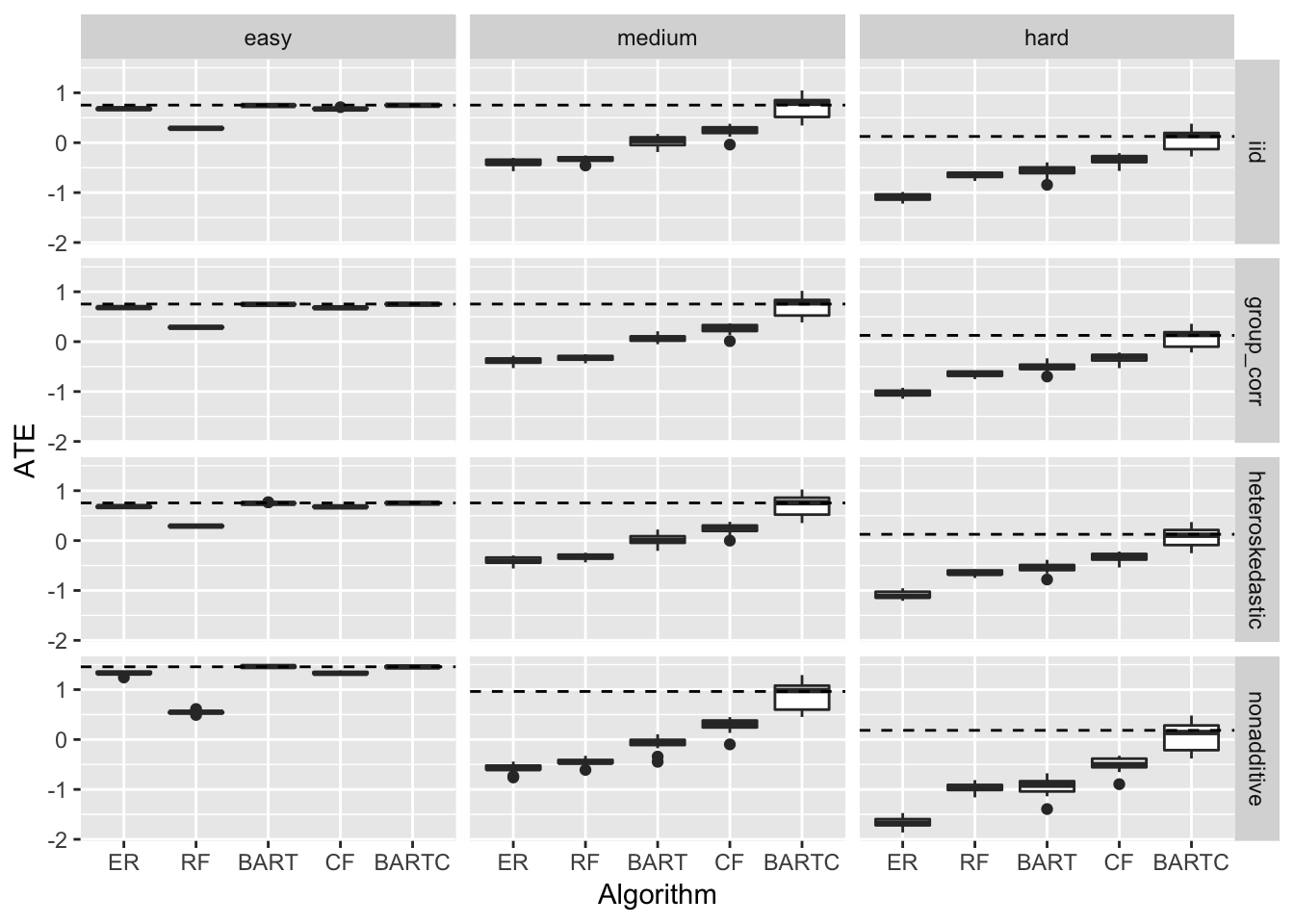
We can see that the error distribution doesn’t change the picture much. For that reason \(RMSE_{ATE}\) figures in the table below are averages over all error distributions:
| algorithm | easy | medium | hard |
|---|---|---|---|
| ER | 0.087 | 1.246 | 1.362 |
| RF | 0.576 | 1.164 | 0.868 |
| BART | 0.003 | 0.798 | 0.779 |
| CF | 0.087 | 0.546 | 0.51 |
| BARTC | 0.001 | 0.038 | 0.052 |
Next thing we can notice is that for the easy case all algorithms nail the \(ATE\) with the exception of RF while for the harder cases they all undershoot by a wide margin with the exception of BARTC which comes pretty close.
CATE
Below I plot \(R^{2}_{CATE}\) box-plots and a red line at 0. We note that while in ML we’d usually think of \(R^{2} = 0\) as the baseline which is equal to “guessing” (since if we guess \(\hat{y}_i = \bar{y} \: \forall \, i\) we get \(R^{2} = 0\)) that wouldn’t be the case in CI. We note that \(\bar{CATE} = ATE\), meaning in CI the equivalent of guessing \(\hat{y}_i = \bar{y} \: \forall \, i\) is guessing \(\hat{CATE}(z) = ATE \: \forall \, z\) and as we saw above that estimating the \(ATE\) isn’t always straight forward.
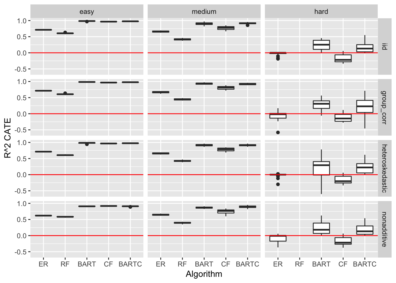
Below I report the resulting average \(\bar{R^{2}}_{CATE}\), averaging over all \(M\) datasets and all error types:
| algorithm | easy | medium | hard |
|---|---|---|---|
| ER | 0.69 | 0.66 | -0.05 |
| RF | 0.6 | 0.42 | -6.77 |
| BART | 0.97 | 0.91 | 0.24 |
| CF | 0.96 | 0.77 | -0.15 |
| BARTC | 0.96 | 0.91 | 0.19 |
We can see that the causal inference oriented algorithms all fair better than the regular ML ones. We can further see that BART and BARTC do best, yet all struggle in the hard case.
Final conclusion
It would seem BART based algorithms are best suited for CI tasks among the competing algorithms. This is not entirely unexpected as it was reported in the past that BART does well for CI tasks. It’s also worth mentioning that the author of the package implementing BARTC is a member of the group that put together the dataset we used in this simulation study.
Think you know an algorithm that can pinpoint the \(CATE\) even in the hard case? You can write them in the comments below, or feel free to use the code that produced this post to add them to the competition.