On my last post I gave an intuitive demonstration of what’s causal inference and how it’s different than classic ML.

After receiving some feedback I realize that while the post was easy to digest, some confusion remains. In this post I’ll delve a bit deeper into what the “causal” in Causal Inference actually means.

Analyzing the effect of X on Y

The field of Causal inference deals with the question of “How does X affect Y?”. While ML practices include procedures that can potentially shed light on the topic, they are generally not well suited to give a concise and correct answer. To see why that’s the case, let’s review how ML is usually used to answer the question “How does X affect Y?”

Partial dependence plots

In classic ML we have some outcome variable \(Y\) for which we’d like to predict the expected outcome given some observed feature set \(\{X,Z\}\):

\[\mathbb{E}(Y|X=x, Z=z)\]

where \(X\) is a feature of special interest (for which we’ll ask “How does X affect Y?”) and \(Z\) are all other measurable features.

Using observations \(\{y_i,x_i,z_i\}, \, i = 1, \dots n\) we construct a predictor function \(f(x,z) = \hat{\mathbb{E}}(Y|X=x,Z=z)\).

When analyzing the marginal effect of a feature of interest \(X\) on the outcome variable \(Y\) the standard practice in ML would be to use partial dependence plots. The partial dependence function is defined as

\[PD(x)=\mathbb{E}(Y|X=x)=\mathbb{E}_Z(f(x,Z))\]

We can see that \(PD(x)\) involves plugging \(x\) to the prediction function \(f\) and marginalizing over the values of the other features \(Z\).

\(PD(x)\) is usually estimated by

\[\hat{PD}(x) = \frac{1}{n}\sum_{i=1}^{n} f(x,z_i)\]

Partial dependence plots (PDP) are then plotted with different values of \(X\) in the x-axis and the corresponding \(PD(x)\) on the y-axis.

A common misconception is thinking that PDP shows how different values of \(X\) affect \(Y\). For example Interpretable ML book states: “The partial dependence plot (short PDP or PD plot) shows the marginal effect one or two features have on the predicted outcome of a machine learning model”.

The kaggle partial dependence plots page states that PDP can answer questions such as “How much of wage differences between men and women are due solely to gender, as opposed to differences in education backgrounds or work experience?” or

“Controlling for house characteristics, what impact do longitude and latitude have on home prices? To restate this, we want to understand how similarly sized houses would be priced in different areas, even if the homes actually at these sites are different sizes.”

To demonstrate why this is a misconception let’s briefly revisit the toy model introduced on my last post:

Imagine we’re tasked by the marketing team to find the effect of raising marketing spend on sales. We have at our disposal records of marketing spend (mkt), visits to our website (visits), sales, and competition index (comp).

We’ll simulate a dataset using a set of equations (also called structural equations):

\[\begin{equation} sales = \beta_1visits + \beta_2comp + \epsilon_1 \end{equation}\] \[\begin{equation} vists = \beta_3mkt + \epsilon_2 \end{equation}\] \[\begin{equation} mkt = \beta_4comp + \epsilon_3 \end{equation}\] \[\begin{equation} comp = \epsilon_4 \end{equation}\]

with \(\{\beta_1, \beta_2, \beta_3\, \beta_4\} = \{0.3, -0.9, 0.5, 0.6\}\) and \(\epsilon_i \sim N(0,1)\)

We can think of the equations above as some data generating process (DGP) underlying our simulated dataset. Let’s label that process \(DGP_{\text{obs}}\) with “obs” standing for “observed”.

Below I generate a sample \(\{sales_i, mkt_i, comp_i, visits_i\}, \, i \in 1, \dots, 10000\) and fit a linear regression model \(sales = r_0 + r_1mkt + r_2visits + r_3comp + \epsilon\) on the first 8000 observations.

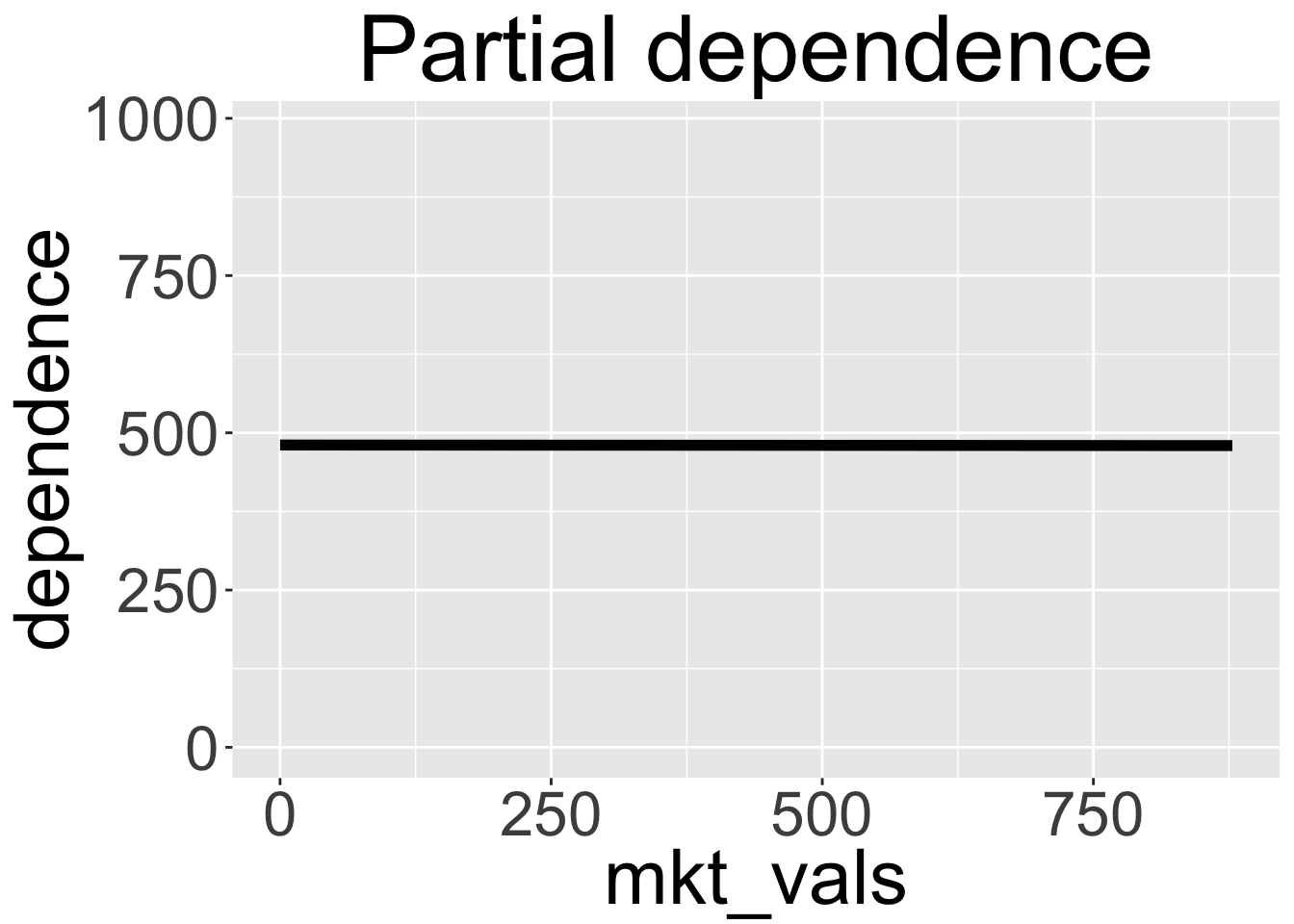
The \(PD\) plot between mkt and sales is shown below:

We can see that the line is essentially flat, indicating no effect, though in fact we know that the line slope should be 0.15 (since \(\beta_1 \cdot \beta_3=0.15\)).

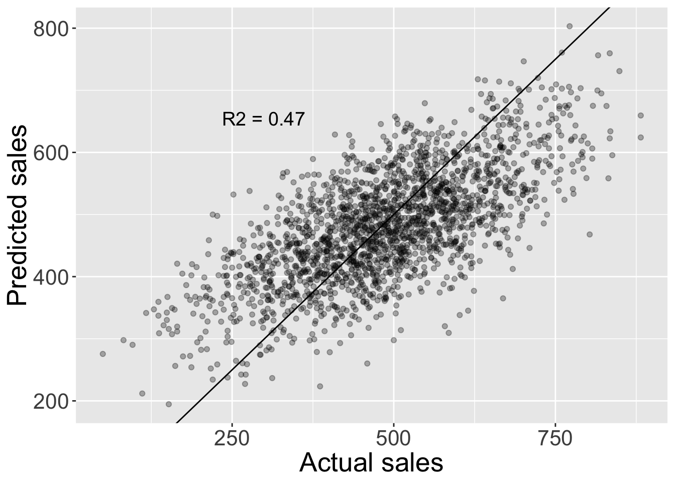
This seems quite surprising (though those who read my last post saw that result where the coefficient for mkt in the full ML model was around 0). The PDP shows none-sense results even though our model, while not perfect does capture a considerable degree of signal as shown in the plot of predicted vs actual sales (in the hold out test set of 2000 observations) below:

The “do” operator

The reason why the relation found was so off is because the question “How does X affect Y” was so far ill defined and so were the tools we used to answer it.

We need to make a distinction between when we observe a feature \(X\) taking some specific value \(x\) in which case we write \(X=x\), and when we “force” or set \(X\) to some value \(x\) in which case we write \(do(X=x)\).

In order to understand the nature of the distinction between observing and setting \(X\) (or \(X=x\) vs \(do(X=x)\)) we first need to understand that by setting \(do(X=x)\) we change how future samples are generated. In our example setting \(do(mkt = x)\) means we delete the 3rd equation above (\(mkt = \beta_4comp + \epsilon_3\)) as mkt is no longer a function of comp. After setting mkt the rest of the variables are generated according to the remaining equations. We arrive at a new data generating process we’ll label \(DGP_{\text{do(mkt = x)}}\) from which samples are generated after we set the mkt value.

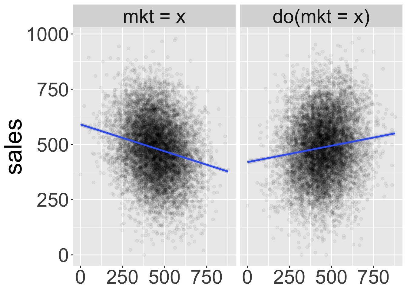
In the plot below I show the a scatter plot of mkt and sales generated by \(DGP_{\text{obs}}\) on the left and those generated by \(DGP_{\text{do(mkt = x)}}\) after setting mkt to different values on the right:

We can see that the joint distribution of mkt and sales is dramatically different before and after setting mkt. When we observe \(mkt=x\) (on the left pane) usually there’s also high competition leading to lower sales. When we set \(do(mkt=x)\) (on the right pane) that is no longer the case and indeed sales increase with mkt as expected. Finding the causal effect in this case does not even require a very complex model: the line slope on the right pane is 0.15 (which is the true causal effect).

The challenge with Causal inference

In causal inference we’re interested in predicting the expected outcome of \(Y\) given we set \(X\) to some value \(x\) and we observed all other features \(Z\) take values \(z\):

\[\mathbb{E}(Y|do(X=x), Z=z)\]

The corresponding causal effect of \(X\) on \(Y\) (defined very similarly to the PD function above) would then be:

\[\mathbb{E}(Y|do(X=x))=\mathbb{E}_Z(Y|do(X=x),Z=z)\]

The hard challenge involved with Causal inference stems from the fact that while \(\mathbb{E}(Y|do(X=x))\) is generated under \(DGP_{\text{do(mkt = x)}}\) we only have observations generated by \(DGP_{\text{obs}}\). That’s because the data generating process would change from \(DGP_{\text{obs}}\) to \(DGP_{\text{do(mkt = x)}}\) only after we set \(do(X=x)\). We need to make predictions on one distribution based on a different distribution. This is very much unlike classic ML where our training sample and outcome variable are both generated by the same distribution.

A further complication that arises from this situation is that we never have ground truth to test our models against. Utilizing ground truth to let models “learn” on their own by trial and error is the corner stone of ML (e.g. using gradient descent to find model parameters).

In ML we can always benchmark how accurate our model \(f(x,z)\) is by fitting it to a train sample and measuring \(L(Y,f(X,Z))\) in the test set (where \(L\) is some loss function representing how far off our model predictions are from the ground truth). We can also benchmark our model to competing models \(f'(x,z)\) without requiring any knowledge about how those models were derived or how their internal machinery works as long as we can compute \(f'(x,z)\).

There’s still hope

While we don’t have observations generated by \(DGP_{\text{do(mkt = x)}}\) there are still instances where we can un-biasedly estimate \(\mathbb{E}(Y|do(X=x))\).

One of those instances happens when we are able to measure a set of variables \(Z_B \subset Z\) that satisfies the “backdoor criteria” (also called “adjustment set”). Roughly this is the set of features that keeps all directed paths between our feature of interest \(X\) and the outcome variable \(Y\) open while blocking any “spurious” paths (See my last post for more details on that).

In the case where we can measure \(Z_B\) we can use the g-computation formula:

\[\mathbb{E}(Y|do(X=x)) = \sum_{z_B}f(x,z_B)P(z_B)\] We note there’s no need to estimate \(P(z_b)\), we can just use samples \(\{y_i,x_i,{z_{B}}_i\}\) to estimate:

\[\mathbb{E}(Y|do(X=x)) = \frac{1}{n}\sum_{i=1}^{n} f(x,z_{B_i})\]

Very much like the \(PD\) function introduced earlier.

In fact we’re back in the good ole’ ML scenario where we can use that shiny new XGBoost implementation and enjoy all the benefits of having ground truth mentioned above as long as we restrict ourselves to using the feature subset \(Z_B\).

All good? not quite

While using the adjustment set \(Z_B\) let’s us use all the mighty good tools we have from ML, it entirely hinges on us constructing the correct data DAG (if you’re not sure what that is, see my last post). Unfortunately that’s not easy to do nor validate.

In future posts I’ll touch upon how to find the correct DAG as well as other complications that usually arise when trying to find causal relations.

"X affects Y". What does that even mean?