Sometimes more data can hurt!

Some context

On a recent blog post I’ve discussed a scalable sparse linear regression model I’ve developed at work. One of it’s interesting properties is that it’s an interpolating model - meaning it has 0-training error. This is because it’s over parameterized and thus can fit the training data perfectly.

While 0-training error is usually associated with over-fiting, the model seems to perform pretty well on the test set. Reports of hugely over-parameterized models that seem to not suffer from overfiting (especially in deep learning) have been accumulating in recent years and so the literature on subject.

My own model for example performs best with no regularization at all. Intrigued by this extraordinary behavior I set out to better understand what’s going on. I got a good intro to the subject in this Medium post.

Since Artificial neural networks are very complex algorithms it’s a good idea to study the subject and build intuition in a simpler setting. This is done in the great paper “More Data Can Hurt for Linear Regression: Sample-wise Double Descent” by Preetum Nakkiran.

I’ll briefly summarize the problem setup: Let’s assume we have data that is generated from a linear model with 1000 covariates (without intercept). For every sample size \(n\) we fit a linear regression and measure the MSE on a hold out test set.

In cases where \(n \geq 1000\) we fit a regular regression model. In cases where \(n<1000\) we have \(p>n\) and there’s no closed form solution since the inverse of the design matrix does not exist.

The equation \(Y=X\beta\) has infinite solutions in this case. Of those solutions, the solution which minimizes the coefficient L2 norm \(||\beta||_2^2\) has the lowest variance and thus should have the best performance on the test set (more on that in Nakkiran’s paper). We can find the minimum norm L2 solution using the Moore-Penrose generalized inverse of a matrix X implemented in the MASS package.

Below we can see the simulation results from the paper: we can see that somewhere around Num. Samples = 900 the test error actually blows up as the number of samples increases towards 1000:

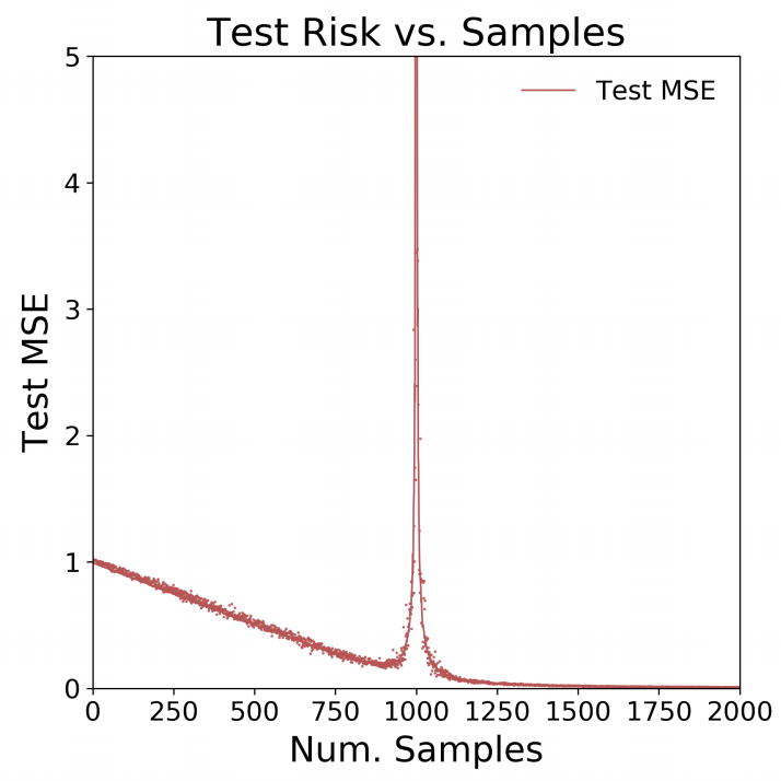
I found that result a bit hard to believe! Worried this may be another case of replication crisis I decided I had to see that for myself. Hence in this post I’ll reproduce the paper results.

Results reproduction

First we setup the simulation parameters:

beta <- runif(1000) # real coefficients
beta <- beta/sqrt(sum(beta^2)) ## convert to a unit vector
M <- 50 ## number of simulations
N <- c(2, seq(100, 800, 100), seq(900, 990, 10), seq(991,1000,1), 
       seq(1001, 1009, 1), seq(1010, 1100, 10), seq(1200, 2000, 100)) ## number of observations
test_MSE <- matrix(nrow = length(N), ncol = M)

Below we perform the actual simulation:

for (i in 1:length(N)){
  for (m in 1:M){
    print(paste0("n=", N[i], ", m=", m))
    # generate traininng data
    X <- replicate(1000, rnorm(N[i]))
    e <- rnorm(N[i], sd = 0.1)
    y <- X %*% beta + e
    
    if (N[i] < 1000){
      beta_hat <- ginv(X) %*% y # Moore-penrose generalized matrix inverse
    } else {
      dat <- as.data.frame(cbind(y, X))
      names(dat)[1] <- "y"
      lm_model <- lm(y ~ .-1, data = dat) # regular fit
      beta_hat <- matrix(lm_model$coefficients, ncol = 1)
    }
    
    # generate test set
    X_test <- replicate(1000, rnorm(10000))
    e_test <- rnorm(10000, sd = 0.1)
    y_test <- X_test %*% beta + e_test
    
    # measure model accuracy
    preds_test <- X_test %*% beta_hat
    test_MSE[i, m] <- sqrt(mean((y_test - preds_test)^2))
  }
}

Let’s plot the results:

matplot(N, test_MSE, type = "p", pch = ".", ylim = c(0,5), 
        xaxt = "n", xlim = c(0,2000), ylab = "Test MSE", xlab = "Num. Samples")
axis(1, at = seq(0,2000,250))
lines(N, apply(test_MSE, 1, mean), col = "red")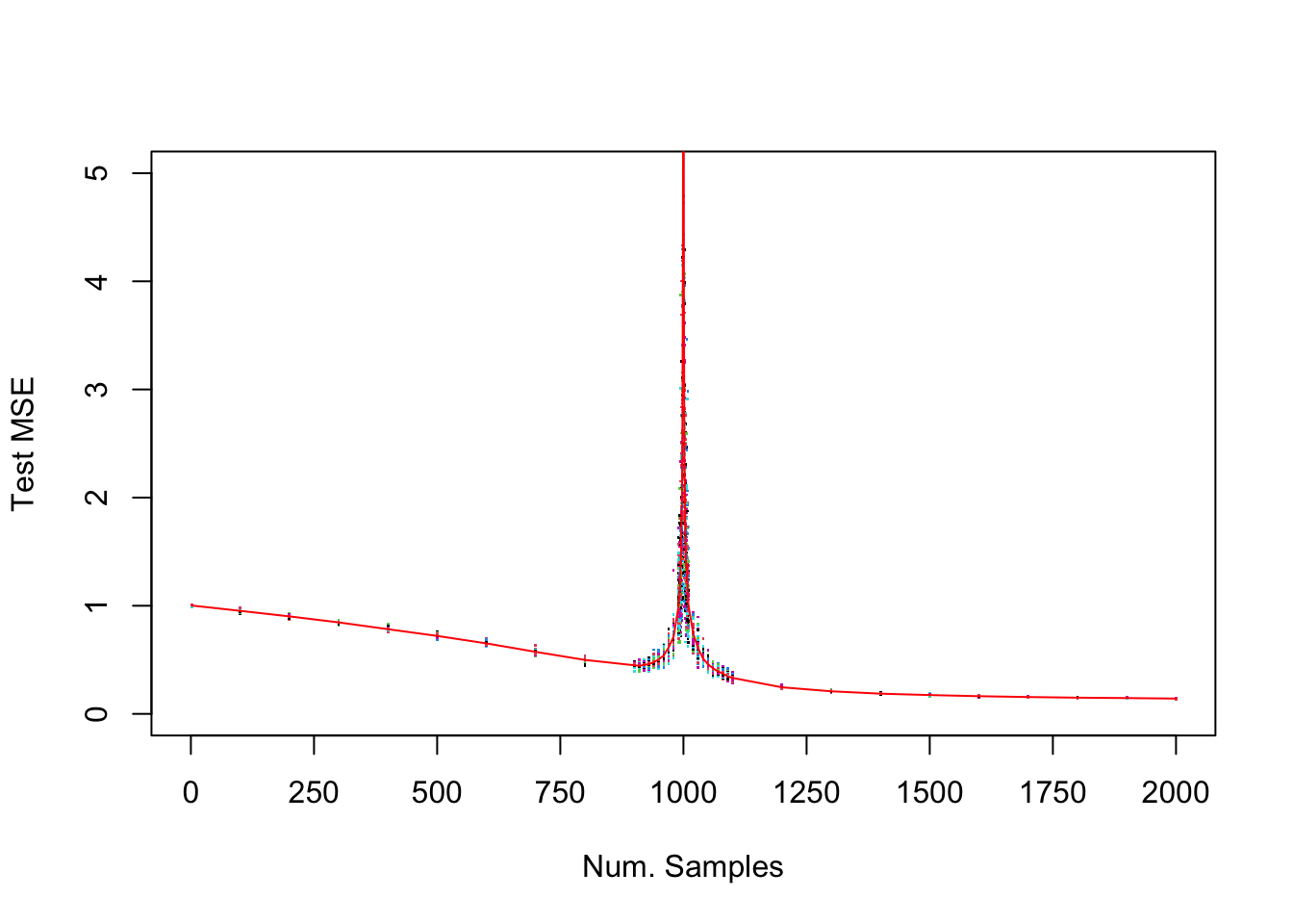

Amazingly enough - we got the exact same results!