It is not often that I find myself thinking “man, I wish we had in R that cool python library!”. That is however the case with the dowhy library which “provides a unified interface for causal inference methods and automatically tests many assumptions, thus making inference accessible to non-experts”.
Luckily enough though, the awesome folks at Rstudio have written the reticulate package just for that sort of occasion: It “provides a comprehensive set of tools for interoperability between Python and R”.
In this post I’ll set about exploring the dowhy library while never leaving my Rstudio IDE or even writing python code!
Below we set up a python virtual environment and install the dowhy dependencies:
# create a new environment
virtualenv_create("r-reticulate")

# install python packages into virtualenv
virtualenv_install("r-reticulate", c("numpy", "scipy", "scikit-learn", "pandas", "dowhy"))
Be sure to use python 3+. If you’re using windows you are out of luck as these support conda environments only and I’m not sure conda support dowhy.
Next, we import the dowhy module right into our R session!
dowhy <- import("dowhy")Now let’s reproduce the first simple example from the dowhy site.
For simplicity, we simulate a dataset with linear relationships between common causes and treatment, and common causes and outcome.
Beta is the true causal effect and is equal to 10. Below we generate the linear dataset:
data <- dowhy$datasets$linear_dataset(
  beta = 10L,
  num_common_causes = 5L,
  num_instruments = 2L,
  num_effect_modifiers = 1L,
  num_samples = 10000L,
  treatment_is_binary = T
)
df_r <- py_to_r(data[["df"]]) # to be used later
Below we can see the first few rows:
data["df"]$df$head() %>% pandoc.table(split.tables = Inf)| X0 | Z0 | Z1 | W0 | W1 | W2 | W3 | W4 | v0 | y |
|---|---|---|---|---|---|---|---|---|---|
| 0.4349 | 0 | 0.6183 | -1.193 | 2.58 | 0.824 | 2.392 | 1.732 | TRUE | 23.05 |
| -0.9587 | 1 | 0.3943 | 0.3835 | 0.371 | -1.838 | 1.835 | 1.867 | TRUE | 11.66 |
| -0.986 | 1 | 0.8709 | -0.0708 | -0.3716 | -0.4343 | 0.2224 | 1.561 | TRUE | 9.258 |
| 0.1813 | 0 | 0.2285 | 0.3961 | 0.1993 | 0.3843 | -0.2072 | -0.6096 | TRUE | 12.79 |
| -0.9915 | 0 | 0.4394 | 0.6585 | -0.5755 | 0.2262 | 1.332 | 0.365 | TRUE | 15.58 |
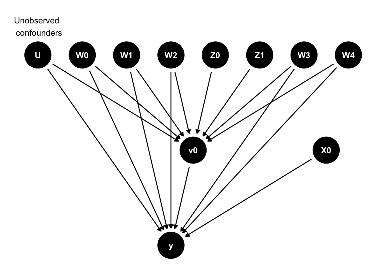
We are interested with estimating the causal effect of \(v0\) (a binary treatment) on \(y\) (10 in this case). The dowhy library streamlines the process of estimating and validating the causal estimate by introducing a flow consisting of 4 key steps. The first is enumerating our assumed causal model, as encoded by a DAG.
1) Enumerate the assumed causal model
The above data object contains the underlying DAG representation. I’ve found that converting dot graphs to dagitty format is pretty straight forward and we’ll use that to plot the graph:
dagitty_graph <- data[["dot_graph"]]
dagitty_graph <- gsub("digraph", "dag", dagitty_graph)
dagitty_graph <- dagitty(dagitty_graph)
# let's arrange the nodes to conform with what is shown in the dowhy example
coordinates(dagitty_graph) <- list(
  x = c(
    U = 0, W0 = 1, W1 = 2, W2 = 3, W3 = 6, W4 = 7,
    X0 = 6.5, Z0 = 4, Z1 = 5, v0 = 3.5, y = 3
  ),
  y = c(
    U = 0, W0 = 0, W1 = 0, W2 = 0, W3 = 0, W4 = 0,
    X0 = -1, Z0 = 0, Z1 = 0, v0 = -1, y = -2
  )
)

ggdag(tidy_dagitty(dagitty_graph)) + theme_dag_blank() +
  annotate(geom = "text", x = 0, y = 0.3, label = "Unobserved \n confounders")
We enumerate the causal model using the following code:
model <- dowhy$CausalModel(
  data = data[["df"]],
  treatment = data[["treatment_name"]],
  outcome = data[["outcome_name"]],
  graph = data[["gml_graph"]]
)
2) Enumerate identification strategies
The next step is enumerating the identification strategies available given the above graph:
identified_estimand <- model$identify_effect(proceed_when_unidentifiable = T)

print(identified_estimand)
## Estimand type: nonparametric-ate
## ### Estimand : 1
## Estimand name: backdoor
## Estimand expression:
## d
## ─────(Expectation(y|W3,W4,W1,W2,W0))
## d[v₀]
## Estimand assumption 1, Unconfoundedness: If U→{v0} and U→y then P(y|v0,W3,W4,W1,W2,W0,U) = P(y|v0,W3,W4,W1,W2,W0)
## ### Estimand : 2
## Estimand name: iv
## Estimand expression:
## Expectation(Derivative(y, [Z1, Z0])*Derivative([v0], [Z1, Z0])**(-1))
## Estimand assumption 1, As-if-random: If U→→y then ¬(U →→{Z1,Z0})
## Estimand assumption 2, Exclusion: If we remove {Z1,Z0}→{v0}, then ¬({Z1,Z0}→y)We can see that there are 2 possible ways of estimating the causal effect: Either using the backdoor criteria or with instrument variables (IV).
We can really see how dowhy does a great job at making causal discovery transparent and explicit in each step of the process.
3) Estimate the causal effect
Next up is doing the actual estimation.
We’ll first try the IV estimand:
causal_estimate <- model$estimate_effect(
  identified_estimand = identified_estimand,
  method_name = "iv.instrumental_variable"
)

print(paste0("Causal Estimate is ", causal_estimate$value))
## [1] "Causal Estimate is 9.64967493839487"Next, let’s try the backdoor estimand, using propensity score stratification:
causal_estimate <- model$estimate_effect(
  identified_estimand = identified_estimand,
  method_name = "backdoor.propensity_score_stratification"
)

print(paste0("Causal Estimate is ", causal_estimate$value))
## [1] "Causal Estimate is 10.1306174998784"4) Validate estimated causal effect
The last step consists of analyzing the level of confidence we have in the estimated causal effect. We’ll proceed with the backdoor estimate.
Let’s start by adding a random (observed) confounder:
res_random <- model$refute_estimate(
  estimand = identified_estimand,
  estimate = causal_estimate,
  method_name = "random_common_cause"
)

print(res_random)
## Refute: Add a Random Common Cause
## Estimated effect:(10.130617499878428,)
## New effect:(10.12114905599205,)We can see the result is pretty stable. This means our sample size (10,000) is probably large enough to accommodate further confounders without loss of accuracy.
Next, let’s see how adding an unobserved confounder can change our estimate. In the code below the effect_strength_on_treatment argument denotes the probability of the confounder flipping the treatment from 0 to 1 (or vice verca). The effect_strength_on_outcome denotes the linear coefficient of the confounder on the outcome.
res_unobserved <- model$refute_estimate(
  estimand = identified_estimand,
  estimate = causal_estimate,
  method_name = "add_unobserved_common_cause",
  confounders_effect_on_treatment = "binary_flip",
  confounders_effect_on_outcome = "linear",
  effect_strength_on_treatment = 0.01,
  effect_strength_on_outcome = 0.02
)

print(res_unobserved)
## Refute: Add an Unobserved Common Cause
## Estimated effect:(10.130617499878428,)
## New effect:(9.452502128579503,)When using the effect strength values given in the example the effect on our estimate seems modest. Let’s try adding a stronger confounder:
res_unobserved <- model$refute_estimate(
  estimand = identified_estimand,
  estimate = causal_estimate,
  method_name = "add_unobserved_common_cause",
  confounders_effect_on_treatment = "binary_flip",
  confounders_effect_on_outcome = "linear",
  effect_strength_on_treatment = 0.05,
  effect_strength_on_outcome = 1
)

print(res_unobserved)
## Refute: Add an Unobserved Common Cause
## Estimated effect:(10.130617499878428,)
## New effect:(5.444774309294754,)It’s pretty surprising to see how bad our estimate would be given a single un-observed confounder with what I’d consider mild confounding effect.
What’s weirder is that the confounder can affect only the treatment (setting effect_strength_on_outcome = 0, essentially making it a non confounder) and still destabilize the estimate in pretty much the same way:
res_unobserved <- model$refute_estimate(
  estimand = identified_estimand,
  estimate = causal_estimate,
  method_name = "add_unobserved_common_cause",
  confounders_effect_on_treatment = "binary_flip",
  confounders_effect_on_outcome = "linear",
  effect_strength_on_treatment = 0.05,
  effect_strength_on_outcome = 0
)

print(res_unobserved)
## Refute: Add an Unobserved Common Cause
## Estimated effect:(10.130617499878428,)
## New effect:(5.67025809685905,)I’ll probably need to research the internal mechanics a bit more to understand how that’s possible.
Let’s try permuting the treatment (making it effectively a placebo) and see how our estimate changes:
res_placebo <- model$refute_estimate(
  estimand = identified_estimand,
  estimate = causal_estimate,
  method_name = "placebo_treatment_refuter",
  placebo_type = "permute"
)

print(res_placebo)
## Refute: Use a Placebo Treatment
## Estimated effect:(10.130617499878428,)
## New effect:(0.1424237753920382,)We can see that the estimated effect is essentially 0, which is what we’d like to see (this means our estimator doesn’t catch random noise as treatment effect).
Finally, let’s see how sensitive is our estimate to removal of 10% of the observations:
res_subset <- model$refute_estimate(
  estimand = identified_estimand,
  estimate = causal_estimate,
  method_name = "data_subset_refuter",
  subset_fraction = 0.9,
  random_seed = 1L
)

print(res_subset)
## Refute: Use a subset of data
## Estimated effect:(10.130617499878428,)
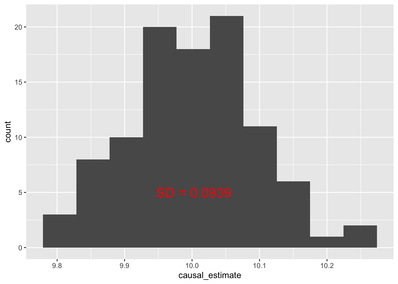
## New effect:(10.05344937871124,)Pretty stable. Thinking about this a bit more I believe this is very similar to using bootstrap sampling to evaluate the estimate variability. Let’s implement bootstrap sampling for variability estimation just for fun:
if (!"res.rds" %in% list.files("../../../")) {
  set.seed(1)
  M <- 100
  res <- vector(length = M)

  for (m in 1:M) {
    bootstarpped_data <- df_r[sample.int(
      n = nrow(df_r),
      nrow(df_r), replace = T
    ), ]

    dat_m <- r_to_py(bootstarpped_data)

    model_m <- dowhy$CausalModel(
      data = dat_m,
      treatment = data[["treatment_name"]],
      outcome = data[["outcome_name"]],
      graph = data[["gml_graph"]]
    )
    identified_estimand <- model_m$identify_effect(
      proceed_when_unidentifiable = T
    )
    causal_estimate <- model_m$estimate_effect(
      identified_estimand = identified_estimand,
      method_name = "backdoor.propensity_score_stratification"
    )
    res[m] <- causal_estimate$value
  }
  saveRDS(res, "../../../res.rds")
} else {
  res <- readRDS("../../../res.rds")
}

res_sd <- round(sd(res), 4)

data.frame(causal_estimate = res) %>%
  ggplot(aes(causal_estimate)) + geom_histogram(bins = 10) +
  annotate(
    geom = "text", x = mean(res), y = 5,
    label = paste0("SD = ", res_sd),
    color = "red", size = 6
  )
Oddly enough it would seem the estimate is pretty far off from 10.
The code above demonstrates how reticulate enables seamless simultaneous coding in Python and R.